セグメンテーション指標の評価

異なるセグメンテーション手法を試す際に、どれが最適かを知るにはどうすればよいでしょうか？ *グランドトゥルース* または *ゴールドスタンダード* セグメンテーションがある場合、さまざまな指標を使用して、各自動化手法がどの程度真実に近いかを確認できます。この例では、セグメント化しやすい画像を使用して、さまざまなセグメンテーション指標の解釈方法を示します。例として、適合Rand誤差と情報の変動を使用し、*過剰セグメンテーション* （真のセグメントを過剰なサブセグメントに分割すること）と *過少セグメンテーション* （異なる真のセグメントを単一のセグメントにマージすること）が異なるスコアにどのように影響するかを確認します。

import numpy as np
import matplotlib.pyplot as plt
from scipy import ndimage as ndi

from skimage import data
from skimage.metrics import adapted_rand_error, variation_of_information
from skimage.filters import sobel
from skimage.measure import label
from skimage.util import img_as_float
from skimage.feature import canny
from skimage.morphology import remove_small_objects
from skimage.segmentation import (
    morphological_geodesic_active_contour,
    inverse_gaussian_gradient,
    watershed,
    mark_boundaries,
)

image = data.coins()

まず、真のセグメンテーションを生成します。この単純な画像の場合、完全なセグメンテーションを生成する正確な関数とパラメータがわかっています。実際のシナリオでは、通常、手動アノテーションまたはセグメンテーションの「ペイント」によってグランドトゥルースを生成します。

elevation_map = sobel(image)
markers = np.zeros_like(image)
markers[image < 30] = 1
markers[image > 150] = 2
im_true = watershed(elevation_map, markers)
im_true = ndi.label(ndi.binary_fill_holes(im_true - 1))[0]

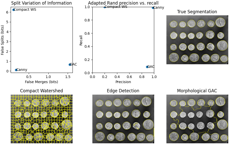
次に、異なる特性を持つ3つの異なるセグメンテーションを作成します。最初のものは、*コンパクトネス* を使用した skimage.segmentation.watershed() を使用します。これは有用な初期セグメンテーションですが、最終結果としては細かすぎます。これが過剰セグメンテーション指標を急上昇させる様子を見ていきます。

edges = sobel(image)
im_test1 = watershed(edges, markers=468, compactness=0.001)

次のアプローチでは、Cannyエッジフィルター skimage.feature.canny() を使用します。これは非常に優れたエッジファインダーであり、バランスの取れた結果をもたらします。

edges = canny(image)
fill_coins = ndi.binary_fill_holes(edges)
im_test2 = ndi.label(remove_small_objects(fill_coins, 21))[0]

最後に、モルフォロジカル測地線アクティブコンター skimage.segmentation.morphological_geodesic_active_contour() を使用します。これは一般的に良好な結果をもたらしますが、適切な解に収束するには長い時間がかかります。意図的に手順を100反復で打ち切っているので、最終結果は *過少セグメント化* されます。つまり、多くの領域が1つのセグメントにマージされます。セグメンテーション指標に対する対応する影響を見ていきます。

image = img_as_float(image)
gradient = inverse_gaussian_gradient(image)
init_ls = np.zeros(image.shape, dtype=np.int8)
init_ls[10:-10, 10:-10] = 1
im_test3 = morphological_geodesic_active_contour(
    gradient,
    num_iter=100,
    init_level_set=init_ls,
    smoothing=1,
    balloon=-1,
    threshold=0.69,
)
im_test3 = label(im_test3)

method_names = [
    'Compact watershed',
    'Canny filter',
    'Morphological Geodesic Active Contours',
]
short_method_names = ['Compact WS', 'Canny', 'GAC']

precision_list = []
recall_list = []
split_list = []
merge_list = []
for name, im_test in zip(method_names, [im_test1, im_test2, im_test3]):
    error, precision, recall = adapted_rand_error(im_true, im_test)
    splits, merges = variation_of_information(im_true, im_test)
    split_list.append(splits)
    merge_list.append(merges)
    precision_list.append(precision)
    recall_list.append(recall)
    print(f'\n## Method: {name}')
    print(f'Adapted Rand error: {error}')
    print(f'Adapted Rand precision: {precision}')
    print(f'Adapted Rand recall: {recall}')
    print(f'False Splits: {splits}')
    print(f'False Merges: {merges}')

fig, axes = plt.subplots(2, 3, figsize=(9, 6), constrained_layout=True)
ax = axes.ravel()

ax[0].scatter(merge_list, split_list)
for i, txt in enumerate(short_method_names):
    ax[0].annotate(txt, (merge_list[i], split_list[i]), verticalalignment='center')
ax[0].set_xlabel('False Merges (bits)')
ax[0].set_ylabel('False Splits (bits)')
ax[0].set_title('Split Variation of Information')

ax[1].scatter(precision_list, recall_list)
for i, txt in enumerate(short_method_names):
    ax[1].annotate(txt, (precision_list[i], recall_list[i]), verticalalignment='center')
ax[1].set_xlabel('Precision')
ax[1].set_ylabel('Recall')
ax[1].set_title('Adapted Rand precision vs. recall')
ax[1].set_xlim(0, 1)
ax[1].set_ylim(0, 1)

ax[2].imshow(mark_boundaries(image, im_true))
ax[2].set_title('True Segmentation')
ax[2].set_axis_off()

ax[3].imshow(mark_boundaries(image, im_test1))
ax[3].set_title('Compact Watershed')
ax[3].set_axis_off()

ax[4].imshow(mark_boundaries(image, im_test2))
ax[4].set_title('Edge Detection')
ax[4].set_axis_off()

ax[5].imshow(mark_boundaries(image, im_test3))
ax[5].set_title('Morphological GAC')
ax[5].set_axis_off()

plt.show()

## Method: Compact watershed
Adapted Rand error: 0.6696040824674964
Adapted Rand precision: 0.19789866776616444
Adapted Rand recall: 0.999747618854942
False Splits: 6.235700763571577
False Merges: 0.10855347108404328

## Method: Canny filter
Adapted Rand error: 0.01477976422795424
Adapted Rand precision: 0.9829789913922441
Adapted Rand recall: 0.9874717238207291
False Splits: 0.11790842956314956
False Merges: 0.17056628682718059

## Method: Morphological Geodesic Active Contours
Adapted Rand error: 0.8380351755097508
Adapted Rand precision: 0.8878701134692834
Adapted Rand recall: 0.08911012454398565
False Splits: 0.6563768831046463
False Merges: 1.5482985465714199