直線ハフ変換

最も単純な形式のハフ変換は、直線を検出する方法です[1]。

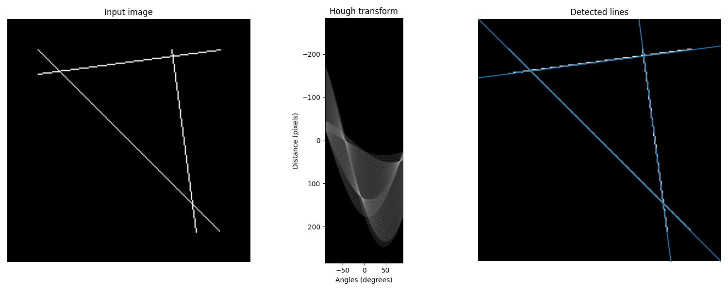
次の例では、直線の交点を持つ画像を構築します。次に、ハフ変換を使用して、画像を通過する可能性のある直線のパラメータ空間を探索します。

アルゴリズムの概要

通常、直線は勾配\(m\)とy切片cを持つ\(y = mx + c\)としてパラメータ化されます。ただし、これは垂直線の場合、\(m\)が無限大になることを意味します。そのため、代わりに、原点につながる線に垂直な線分を構築します。線はその線分の長さ\(r\)とx軸との角度\(\theta\)で表されます。

ハフ変換は、パラメータ空間（つまり、半径の\(M\)個の異なる値と\(\theta\)の\(N\)個の異なる値に対する\(M \times N\)行列）を表すヒストグラム配列を構築します。各パラメータの組み合わせ\(r\)と\(\theta\)について、対応する直線の近くに収まる入力画像内の非ゼロピクセル数を見つけ、位置\((r, \theta)\)の配列を適切に増分します。

各非ゼロピクセルが潜在的な直線の候補に「投票」していると考えることができます。結果のヒストグラムの局所的最大値は、最も可能性の高い直線のパラメータを示します。この例では、最大値は45度と135度で発生し、各直線の法線ベクトル角度に対応します。

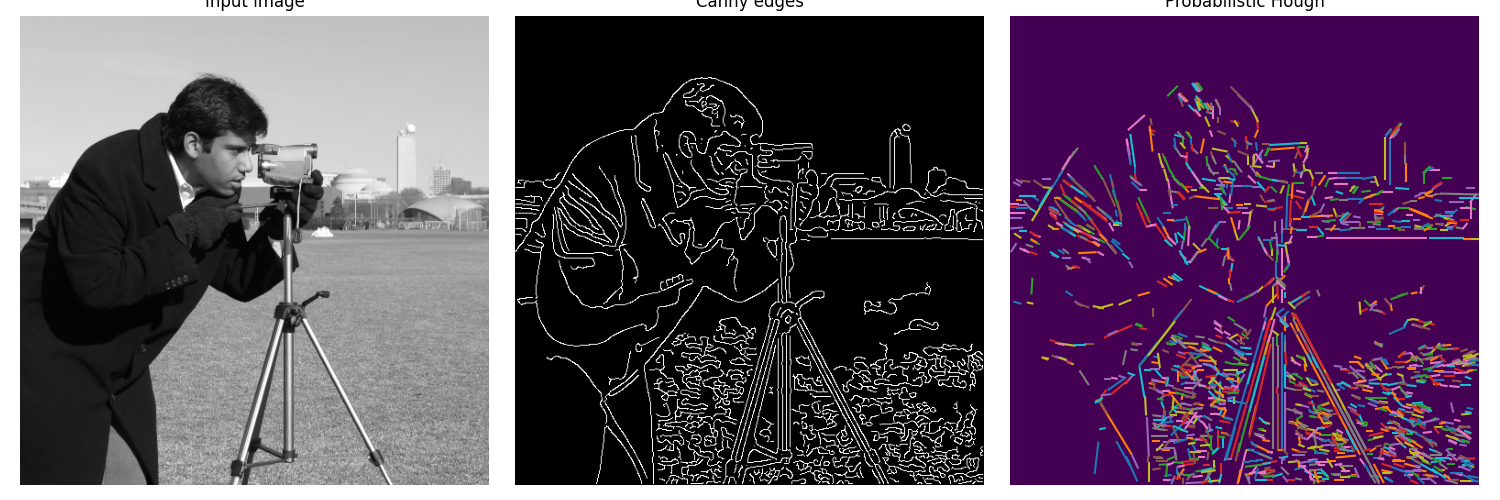
別のアプローチは、プログレッシブ確率的ハフ変換です[2]。これは、投票ポイントのランダムなサブセットを使用すると、実際の結果に良好な近似が得られ、接続されたコンポーネントに沿って歩くことで投票プロセス中に線を抽出できるという仮定に基づいています。これは、各線分の開始と終了を返します。これは便利です。

関数probabilistic_houghには3つのパラメータがあります。ハフアキュムレータに適用される一般的なしきい値、最小線長、および線マージに影響を与える線ギャップです。以下の例では、ギャップが3ピクセル未満の10より長い線を見つけます。

参考文献

[1]

Duda、R。O.およびP.E.Hart、「画像内の線と曲線を検出するためのハフ変換の使用」、Comm。ACM、Vol。15、pp.11-15（1972年1月）

[2]

C.Galamhos、J.Matas、J.Kittler、「線検出のためのプログレッシブ確率的ハフ変換」、IEEE Computer Society Conference on Computer Vision and Pattern Recognition、1999。

線ハフ変換

import numpy as np

from skimage.transform import hough_line, hough_line_peaks
from skimage.feature import canny
from skimage.draw import line as draw_line
from skimage import data

import matplotlib.pyplot as plt
from matplotlib import cm


# Constructing test image
image = np.zeros((200, 200))
idx = np.arange(25, 175)
image[idx, idx] = 255
image[draw_line(45, 25, 25, 175)] = 255
image[draw_line(25, 135, 175, 155)] = 255

# Classic straight-line Hough transform
# Set a precision of 0.5 degree.
tested_angles = np.linspace(-np.pi / 2, np.pi / 2, 360, endpoint=False)
h, theta, d = hough_line(image, theta=tested_angles)

# Generating figure 1
fig, axes = plt.subplots(1, 3, figsize=(15, 6))
ax = axes.ravel()

ax[0].imshow(image, cmap=cm.gray)
ax[0].set_title('Input image')
ax[0].set_axis_off()

angle_step = 0.5 * np.diff(theta).mean()
d_step = 0.5 * np.diff(d).mean()
bounds = [
    np.rad2deg(theta[0] - angle_step),
    np.rad2deg(theta[-1] + angle_step),
    d[-1] + d_step,
    d[0] - d_step,
]
ax[1].imshow(np.log(1 + h), extent=bounds, cmap=cm.gray, aspect=1 / 1.5)
ax[1].set_title('Hough transform')
ax[1].set_xlabel('Angles (degrees)')
ax[1].set_ylabel('Distance (pixels)')
ax[1].axis('image')

ax[2].imshow(image, cmap=cm.gray)
ax[2].set_ylim((image.shape[0], 0))
ax[2].set_axis_off()
ax[2].set_title('Detected lines')

for _, angle, dist in zip(*hough_line_peaks(h, theta, d)):
    (x0, y0) = dist * np.array([np.cos(angle), np.sin(angle)])
    ax[2].axline((x0, y0), slope=np.tan(angle + np.pi / 2))

plt.tight_layout()
plt.show()

確率的ハフ変換

from skimage.transform import probabilistic_hough_line

# Line finding using the Probabilistic Hough Transform
image = data.camera()
edges = canny(image, 2, 1, 25)
lines = probabilistic_hough_line(edges, threshold=10, line_length=5, line_gap=3)

# Generating figure 2
fig, axes = plt.subplots(1, 3, figsize=(15, 5), sharex=True, sharey=True)
ax = axes.ravel()

ax[0].imshow(image, cmap=cm.gray)
ax[0].set_title('Input image')

ax[1].imshow(edges, cmap=cm.gray)
ax[1].set_title('Canny edges')

ax[2].imshow(edges * 0)
for line in lines:
    p0, p1 = line
    ax[2].plot((p0[0], p1[0]), (p0[1], p1[1]))
ax[2].set_xlim((0, image.shape[1]))
ax[2].set_ylim((image.shape[0], 0))
ax[2].set_title('Probabilistic Hough')

for a in ax:
    a.set_axis_off()

plt.tight_layout()
plt.show()