注記
完全なサンプルコードをダウンロードするには、最後まで進むか、Binder を介してブラウザでこの例を実行してください。
ラドン変換#
コンピュータ断層撮影では、断層撮影再構成問題は、一連の投影から断層断面画像を取得することです[1]。投影は、対象の 2 次元オブジェクトに一連の平行光線を描き、各光線に沿ったオブジェクトのコントラストの積分を投影内の単一ピクセルに割り当てることによって形成されます。2 次元オブジェクトの単一投影は 1 次元です。オブジェクトのコンピュータ断層撮影再構成を可能にするには、複数の投影を取得する必要があり、それぞれがオブジェクトに対する光線の異なる角度に対応しています。複数角度での投影の集合は、サイノグラムと呼ばれ、元の画像の線形変換です。
逆ラドン変換は、コンピュータ断層撮影において、測定された投影(サイノグラム)から 2 次元画像を再構成するために使用されます。逆ラドン変換の実用的な厳密な実装は存在しませんが、いくつかの優れた近似アルゴリズムが利用可能です。
逆ラドン変換は一連の投影からオブジェクトを再構成するため、(順方向)ラドン変換は断層撮影実験のシミュレーションに使用できます。
このスクリプトは、断層撮影実験をシミュレートするためにラドン変換を実行し、シミュレーションによって形成された結果のサイノグラムに基づいて入力画像を再構成します。逆ラドン変換を実行して元の画像を再構成する 2 つの方法、フィルタ逆投影 (FBP) と同時代数的再構成手法 (SART) が比較されます。
断層撮影再構成の詳細については、以下を参照してください。
順変換#
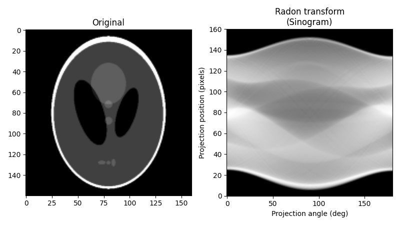
元の画像として、Shepp-Logan ファントムを使用します。ラドン変換を計算する場合、使用する投影角度の数を決定する必要があります。経験則として、投影の数はオブジェクト全体のピクセル数とほぼ同じである必要があります(これがそうである理由を確認するには、再構成プロセスで決定する必要がある未知のピクセル値の数を考慮し、これを投影によって提供される測定値の数と比較してください)、ここではその規則に従います。以下は元の画像とそのラドン変換であり、多くの場合、*サイノグラム*として知られています。
import numpy as np
import matplotlib.pyplot as plt

from skimage.data import shepp_logan_phantom
from skimage.transform import radon, rescale

image = shepp_logan_phantom()
image = rescale(image, scale=0.4, mode='reflect', channel_axis=None)

fig, (ax1, ax2) = plt.subplots(1, 2, figsize=(8, 4.5))

ax1.set_title("Original")
ax1.imshow(image, cmap=plt.cm.Greys_r)

theta = np.linspace(0.0, 180.0, max(image.shape), endpoint=False)
sinogram = radon(image, theta=theta)
dx, dy = 0.5 * 180.0 / max(image.shape), 0.5 / sinogram.shape[0]
ax2.set_title("Radon transform\n(Sinogram)")
ax2.set_xlabel("Projection angle (deg)")
ax2.set_ylabel("Projection position (pixels)")
ax2.imshow(
    sinogram,
    cmap=plt.cm.Greys_r,
    extent=(-dx, 180.0 + dx, -dy, sinogram.shape[0] + dy),
    aspect='auto',
)

fig.tight_layout()
plt.show()
フィルタ逆投影 (FBP) を使用した再構成#
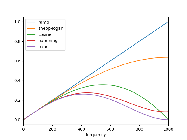
フィルタ逆投影の数学的基礎は、フーリエスライス定理です[2]。投影のフーリエ変換とフーリエ空間での補間を使用して、画像の 2 次元フーリエ変換を取得し、それを反転して再構成された画像を形成します。フィルタ逆投影は、逆ラドン変換を実行する最速の方法の 1 つです。FBP の唯一の調整可能なパラメータはフィルタであり、フーリエ変換された投影に適用されます。再構成における高周波ノイズを抑制するために使用できます。skimage は、「ランプ」、「シェップローガン」、「コサイン」、「ハミング」、および「ハン」フィルタを提供します。
import matplotlib.pyplot as plt
from skimage.transform.radon_transform import _get_fourier_filter

filters = ['ramp', 'shepp-logan', 'cosine', 'hamming', 'hann']

for ix, f in enumerate(filters):
    response = _get_fourier_filter(2000, f)
    plt.plot(response, label=f)

plt.xlim([0, 1000])
plt.xlabel('frequency')
plt.legend()
plt.show()
「ランプ」フィルタを使用して逆ラドン変換を適用すると、次のようになります。
from skimage.transform import iradon

reconstruction_fbp = iradon(sinogram, theta=theta, filter_name='ramp')
error = reconstruction_fbp - image
print(f'FBP rms reconstruction error: {np.sqrt(np.mean(error**2)):.3g}')

imkwargs = dict(vmin=-0.2, vmax=0.2)
fig, (ax1, ax2) = plt.subplots(1, 2, figsize=(8, 4.5), sharex=True, sharey=True)
ax1.set_title("Reconstruction\nFiltered back projection")
ax1.imshow(reconstruction_fbp, cmap=plt.cm.Greys_r)
ax2.set_title("Reconstruction error\nFiltered back projection")
ax2.imshow(reconstruction_fbp - image, cmap=plt.cm.Greys_r, **imkwargs)
plt.show()
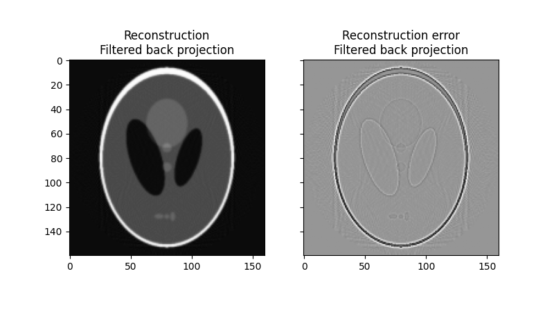
FBP rms reconstruction error: 0.0283
同時代数的再構成手法を使用した再構成#
断層撮影のための代数的再構成手法は、単純な考えに基づいています。ピクセル化された画像の場合、特定の投影における単一光線の値は、光線がオブジェクトを通過する際に通過するすべてのピクセルの合計にすぎません。これは、順方向ラドン変換を表現する方法です。逆ラドン変換は、(大規模な)線形方程式系として定式化できます。各光線は画像内のピクセルのほんの一部を通過するため、この方程式系はスパースであり、スパース線形系のための反復ソルバーが方程式系に取り組むことができます。1 つの反復法、つまり Kaczmarz 法[3]が特に人気があり、解が方程式系の最小二乗解に近づくという特性があります。
再構成問題を線形方程式系と反復ソルバーとして定式化することで、代数的手法は比較的柔軟になり、そのため、ある形式の事前知識を比較的簡単に組み込むことができます。
skimageは、代数的再構成手法の中でも広く利用されている手法の1つである同時代数的再構成手法(SART)を提供しています[4]。これは、反復ソルバーとしてKaczmarz法を使用します。通常、1回の反復で良好な再構成が得られるため、計算効率の高い方法です。1回以上の追加反復を実行すると、通常、シャープな高周波 features の再構成が改善され、平均二乗誤差が減少しますが、高周波ノイズが増加します(ユーザーは、手元の問題に最適な反復回数を決める必要があります)。skimageの実装では、再構成値の下限と上限のしきい値という形式の事前情報を再構成に提供できます。
from skimage.transform import iradon_sart

reconstruction_sart = iradon_sart(sinogram, theta=theta)
error = reconstruction_sart - image
print(
    f'SART (1 iteration) rms reconstruction error: ' f'{np.sqrt(np.mean(error**2)):.3g}'
)

fig, axes = plt.subplots(2, 2, figsize=(8, 8.5), sharex=True, sharey=True)
ax = axes.ravel()

ax[0].set_title("Reconstruction\nSART")
ax[0].imshow(reconstruction_sart, cmap=plt.cm.Greys_r)

ax[1].set_title("Reconstruction error\nSART")
ax[1].imshow(reconstruction_sart - image, cmap=plt.cm.Greys_r, **imkwargs)

# Run a second iteration of SART by supplying the reconstruction
# from the first iteration as an initial estimate
reconstruction_sart2 = iradon_sart(sinogram, theta=theta, image=reconstruction_sart)
error = reconstruction_sart2 - image
print(
    f'SART (2 iterations) rms reconstruction error: '
    f'{np.sqrt(np.mean(error**2)):.3g}'
)

ax[2].set_title("Reconstruction\nSART, 2 iterations")
ax[2].imshow(reconstruction_sart2, cmap=plt.cm.Greys_r)

ax[3].set_title("Reconstruction error\nSART, 2 iterations")
ax[3].imshow(reconstruction_sart2 - image, cmap=plt.cm.Greys_r, **imkwargs)
plt.show()
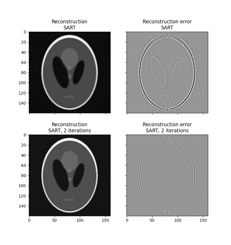
SART (1 iteration) rms reconstruction error: 0.0329
SART (2 iterations) rms reconstruction error: 0.0214
スクリプトの総実行時間:(0分2.276秒)