バターワースフィルタ

バターワースフィルタは周波数領域で実装され、パスバンドまたはストップバンドリップルを持たないように設計されています。ローパスまたはハイパスバリアントのいずれかで使用する事ができます。cutoff_frequency_ratioパラメータを使用して、サンプリング周波数の分数としてカットオフ周波数を設定します。ナイキスト周波数はサンプリング周波数の半分であるため、このパラメータは0.5未満の正の浮動小数点値である必要があります。orderフィルタの次数を調整して遷移幅を制御できます。値が高いほど、パスバンドとストップバンド間の遷移がシャープになります。

バターワースフィルタリングの例

ここでは、指定された一連のカットオフ周波数でローパスフィルタリングとハイパスフィルタリングを繰り返すget_filteredヘルパー関数を定義します。

import matplotlib.pyplot as plt

from skimage import data, filters

image = data.camera()

# cutoff frequencies as a fraction of the maximum frequency
cutoffs = [0.02, 0.08, 0.16]


def get_filtered(image, cutoffs, squared_butterworth=True, order=3.0, npad=0):
    """Lowpass and highpass butterworth filtering at all specified cutoffs.

    Parameters
    ----------
    image : ndarray
        The image to be filtered.
    cutoffs : sequence of int
        Both lowpass and highpass filtering will be performed for each cutoff
        frequency in `cutoffs`.
    squared_butterworth : bool, optional
        Whether the traditional Butterworth filter or its square is used.
    order : float, optional
        The order of the Butterworth filter

    Returns
    -------
    lowpass_filtered : list of ndarray
        List of images lowpass filtered at the frequencies in `cutoffs`.
    highpass_filtered : list of ndarray
        List of images highpass filtered at the frequencies in `cutoffs`.
    """

    lowpass_filtered = []
    highpass_filtered = []
    for cutoff in cutoffs:
        lowpass_filtered.append(
            filters.butterworth(
                image,
                cutoff_frequency_ratio=cutoff,
                order=order,
                high_pass=False,
                squared_butterworth=squared_butterworth,
                npad=npad,
            )
        )
        highpass_filtered.append(
            filters.butterworth(
                image,
                cutoff_frequency_ratio=cutoff,
                order=order,
                high_pass=True,
                squared_butterworth=squared_butterworth,
                npad=npad,
            )
        )
    return lowpass_filtered, highpass_filtered


def plot_filtered(lowpass_filtered, highpass_filtered, cutoffs):
    """Generate plots for paired lists of lowpass and highpass images."""
    fig, axes = plt.subplots(2, 1 + len(cutoffs), figsize=(12, 8))
    fontdict = dict(fontsize=14, fontweight='bold')

    axes[0, 0].imshow(image, cmap='gray')
    axes[0, 0].set_title('original', fontdict=fontdict)
    axes[1, 0].set_axis_off()

    for i, c in enumerate(cutoffs):
        axes[0, i + 1].imshow(lowpass_filtered[i], cmap='gray')
        axes[0, i + 1].set_title(f'lowpass, c={c}', fontdict=fontdict)
        axes[1, i + 1].imshow(highpass_filtered[i], cmap='gray')
        axes[1, i + 1].set_title(f'highpass, c={c}', fontdict=fontdict)

    for ax in axes.ravel():
        ax.set_xticks([])
        ax.set_yticks([])
    plt.tight_layout()
    return fig, axes


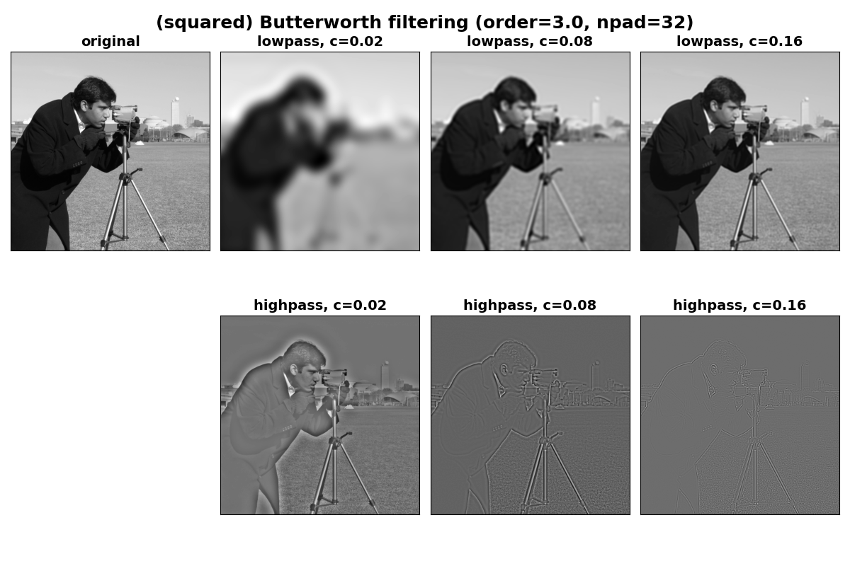
# Perform filtering with the (squared) Butterworth filter at a range of
# cutoffs.
lowpasses, highpasses = get_filtered(image, cutoffs, squared_butterworth=True)

fig, axes = plot_filtered(lowpasses, highpasses, cutoffs)
titledict = dict(fontsize=18, fontweight='bold')
fig.text(
    0.5,
    0.95,
    '(squared) Butterworth filtering (order=3.0, npad=0)',
    fontdict=titledict,
    horizontalalignment='center',
)

Text(0.5, 0.95, '(squared) Butterworth filtering (order=3.0, npad=0)')

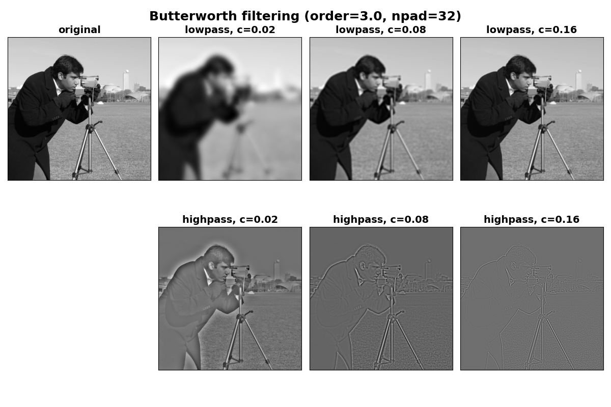
境界アーティファクトの回避

上記の画像では、画像の端の近くにアーティファクト（特に小さなカットオフ値の場合）があることがわかります。これはDFTの周期的な性質によるものであり、フィルタリングの前に端に追加のパディングを適用することで軽減できます。これにより、画像の周期的な拡張にシャープなエッジがなくなります。これは、butterworthのnpad引数を使用することで行うことができます。

パディングを使用すると、画像の端にある望ましくないシェーディングが大幅に軽減されることに注意してください。

lowpasses, highpasses = get_filtered(image, cutoffs, squared_butterworth=True, npad=32)

fig, axes = plot_filtered(lowpasses, highpasses, cutoffs)
fig.text(
    0.5,
    0.95,
    '(squared) Butterworth filtering (order=3.0, npad=32)',
    fontdict=titledict,
    horizontalalignment='center',
)

Text(0.5, 0.95, '(squared) Butterworth filtering (order=3.0, npad=32)')

真のバターワースフィルタ

従来の信号処理におけるバターワースフィルタの定義を使用するには、squared_butterworth=Falseを設定します。このバリアントは、周波数領域における振幅プロファイルがデフォルトケースの平方根になります。これにより、指定されたorderで、パスバンドからストップバンドへの遷移がより緩やかになります。これは、上記の平方バターワースに対応するものよりもローパスケースで少しシャープに見える次の画像で確認できます。

lowpasses, highpasses = get_filtered(image, cutoffs, squared_butterworth=False, npad=32)

fig, axes = plot_filtered(lowpasses, highpasses, cutoffs)
fig.text(
    0.5,
    0.95,
    'Butterworth filtering (order=3.0, npad=32)',
    fontdict=titledict,
    horizontalalignment='center',
)

plt.show()