領域プロパティの測定

この例では、ラベル付けされた画像領域のプロパティを測定する方法を示します。最初に、2つの楕円を持つ画像を分析します。以下では、ラベル付けされたオブジェクトのプロパティをインタラクティブに探索する方法を示します。

import math
import matplotlib.pyplot as plt
import numpy as np
import pandas as pd

from skimage.draw import ellipse
from skimage.measure import label, regionprops, regionprops_table
from skimage.transform import rotate


image = np.zeros((600, 600))

rr, cc = ellipse(300, 350, 100, 220)
image[rr, cc] = 1

image = rotate(image, angle=15, order=0)

rr, cc = ellipse(100, 100, 60, 50)
image[rr, cc] = 1

label_img = label(image)
regions = regionprops(label_img)

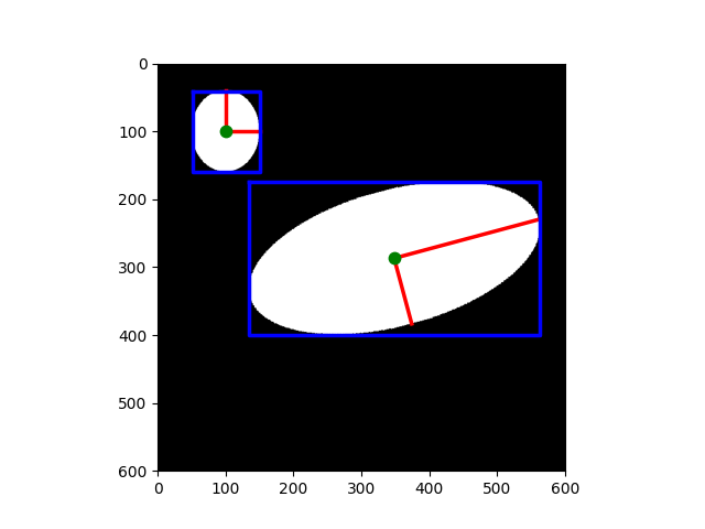
skimage.measure.regionprops() の結果を使用して、各領域に特定のプロパティを描画します。たとえば、赤で各楕円の主軸と副軸をプロットします。

fig, ax = plt.subplots()
ax.imshow(image, cmap=plt.cm.gray)

for props in regions:
    y0, x0 = props.centroid
    orientation = props.orientation
    x1 = x0 + math.cos(orientation) * 0.5 * props.axis_minor_length
    y1 = y0 - math.sin(orientation) * 0.5 * props.axis_minor_length
    x2 = x0 - math.sin(orientation) * 0.5 * props.axis_major_length
    y2 = y0 - math.cos(orientation) * 0.5 * props.axis_major_length

    ax.plot((x0, x1), (y0, y1), '-r', linewidth=2.5)
    ax.plot((x0, x2), (y0, y2), '-r', linewidth=2.5)
    ax.plot(x0, y0, '.g', markersize=15)

    minr, minc, maxr, maxc = props.bbox
    bx = (minc, maxc, maxc, minc, minc)
    by = (minr, minr, maxr, maxr, minr)
    ax.plot(bx, by, '-b', linewidth=2.5)

ax.axis((0, 600, 600, 0))
plt.show()

skimage.measure.regionprops_table() 関数を使用して、各領域の（選択された）プロパティを計算します。skimage.measure.regionprops_table は実際にプロパティを計算しますが、skimage.measure.regionprops は使用時にプロパティを計算する（遅延評価）ことに注意してください。

props = regionprops_table(
    label_img,
    properties=('centroid', 'orientation', 'axis_major_length', 'axis_minor_length'),
)

ここで、これらの選択されたプロパティのテーブルを表示します（行ごとに1つの領域）。skimage.measure.regionprops_table の結果は、pandas互換の辞書です。

pd.DataFrame(props)

	重心-0	重心-1	方向	長軸の長さ	短軸の長さ
0	100.000000	100.000000	0.000000	119.807049	99.823995
1	286.914167	348.412995	-1.308966	440.015503	199.918850

ラベルのホバー情報にラベル付けされたオブジェクトのプロパティを視覚化することにより、インタラクティブに探索することもできます。この例では、オブジェクトにカーソルを合わせたときにプロパティを表示するためにplotlyを使用しています。

import plotly
import plotly.express as px
import plotly.graph_objects as go
from skimage import data, filters, measure, morphology

img = data.coins()
# Binary image, post-process the binary mask and compute labels
threshold = filters.threshold_otsu(img)
mask = img > threshold
mask = morphology.remove_small_objects(mask, 50)
mask = morphology.remove_small_holes(mask, 50)
labels = measure.label(mask)

fig = px.imshow(img, binary_string=True)
fig.update_traces(hoverinfo='skip')  # hover is only for label info

props = measure.regionprops(labels, img)
properties = ['area', 'eccentricity', 'perimeter', 'intensity_mean']

# For each label, add a filled scatter trace for its contour,
# and display the properties of the label in the hover of this trace.
for index in range(1, labels.max()):
    label_i = props[index].label
    contour = measure.find_contours(labels == label_i, 0.5)[0]
    y, x = contour.T
    hoverinfo = ''
    for prop_name in properties:
        hoverinfo += f'<b>{prop_name}: {getattr(props[index], prop_name):.2f}</b><br>'
    fig.add_trace(
        go.Scatter(
            x=x,
            y=y,
            name=label_i,
            mode='lines',
            fill='toself',
            showlegend=False,
            hovertemplate=hoverinfo,
            hoveron='points+fills',
        )
    )

plotly.io.show(fig)