核膜での蛍光強度測定

この例では、細胞画像の時間シーケンス（それぞれ2つのチャネルと2つの空間次元を持つ）で、核膜に局在する蛍光強度を測定するための、バイオイメージデータ解析における確立されたワークフローを再現します。この時間シーケンスは、細胞質領域から核膜へのタンパク質の再局在の過程を示しています。この生物学的応用は、Andrea Boniとその共同研究者によって最初に発表され[1]、Kota Miuraの教科書[2]やその他の研究（[3], [4]）でも使用されました。言い換えれば、このワークフローをImageJマクロからscikit-imageを使用したPythonに移植します。

[1]

Boni A, Politi AZ, Strnad P, Xiang W, Hossain MJ, Ellenberg J (2015) “Live imaging and modeling of inner nuclear membrane targeting reveals its molecular requirements in mammalian cells” J Cell Biol 209(5):705–720. ISSN: 0021-9525. DOI:10.1083/jcb.201409133

[2]

Miura K (2020) “Measurements of Intensity Dynamics at the Periphery of the Nucleus” in: Miura K, Sladoje N (eds) Bioimage Data Analysis Workflows. Learning Materials in Biosciences. Springer, Cham. DOI:10.1007/978-3-030-22386-1_2

[3]

Klemm A (2020) “ImageJ/Fiji Macro Language” NEUBIAS Academy Online Course: https://www.youtube.com/watch?v=o8tfkdcd3DA

[4]

Vorkel D and Haase R (2020) “GPU-accelerating ImageJ Macro image processing workflows using CLIJ” https://arxiv.org/abs/2008.11799

import matplotlib.pyplot as plt
import numpy as np
import plotly.io
import plotly.express as px
from scipy import ndimage as ndi

from skimage import filters, measure, morphology, segmentation
from skimage.data import protein_transport

まず、ワークフローを構築するために、単一の細胞/核から始めます。

image_sequence = protein_transport()

print(f'shape: {image_sequence.shape}')

shape: (15, 2, 180, 183)

データセットは、15フレーム（時間点）と2チャネルを持つ2D画像スタックです。

vmin, vmax = 0, image_sequence.max()

fig = px.imshow(
    image_sequence,
    facet_col=1,
    animation_frame=0,
    zmin=vmin,
    zmax=vmax,
    binary_string=True,
    labels={'animation_frame': 'time point', 'facet_col': 'channel'},
)
plotly.io.show(fig)

まず、最初の画像の最初のチャネルを考慮しましょう（下の図のステップa)）。

image_t_0_channel_0 = image_sequence[0, 0, :, :]

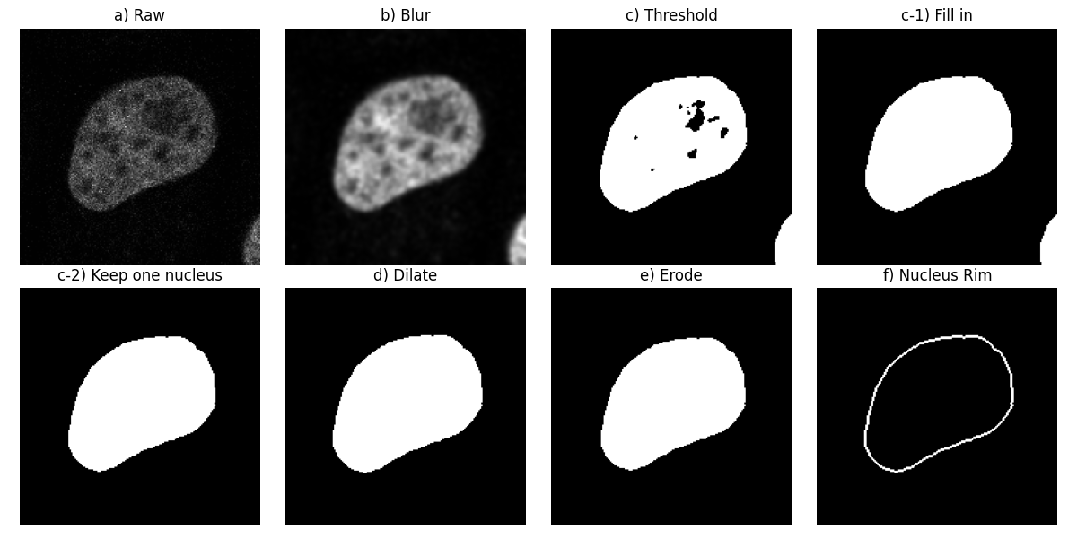
核の縁のセグメンテーション

この画像を平滑化するために、ガウスローパスフィルターを適用しましょう（ステップb)）。次に、大津の方法を使用して、バックグラウンドとフォアグラウンドの間の閾値を見つけて核をセグメンテーションします。これにより、バイナリ画像を取得します（ステップc)）。次に、オブジェクト内の穴を埋めます（ステップc-1)）。

smooth = filters.gaussian(image_t_0_channel_0, sigma=1.5)

thresh_value = filters.threshold_otsu(smooth)
thresh = smooth > thresh_value

fill = ndi.binary_fill_holes(thresh)

元のワークフローに従って、画像の境界に触れるオブジェクトを削除しましょう（ステップc-2)）。ここでは、別の核の一部が右下の隅に触れていることがわかります。

clear = segmentation.clear_border(fill)
clear.dtype

dtype('bool')

このバイナリ画像のモルフォロジー膨張（ステップd)）とそのモルフォロジー侵食（ステップe)）の両方を計算します。

dilate = morphology.binary_dilation(clear)

erode = morphology.binary_erosion(clear)

最後に、核の縁を取得するために、膨張した画像から侵食した画像を減算します（ステップf)）。これは、dilateにあり、erodeにはないピクセルを選択することと同じです。

mask = np.logical_and(dilate, ~erode)

これらの処理ステップをサブプロットのシーケンスで視覚化しましょう。

fig, ax = plt.subplots(2, 4, figsize=(12, 6), sharey=True)

ax[0, 0].imshow(image_t_0_channel_0, cmap=plt.cm.gray)
ax[0, 0].set_title('a) Raw')

ax[0, 1].imshow(smooth, cmap=plt.cm.gray)
ax[0, 1].set_title('b) Blur')

ax[0, 2].imshow(thresh, cmap=plt.cm.gray)
ax[0, 2].set_title('c) Threshold')

ax[0, 3].imshow(fill, cmap=plt.cm.gray)
ax[0, 3].set_title('c-1) Fill in')

ax[1, 0].imshow(clear, cmap=plt.cm.gray)
ax[1, 0].set_title('c-2) Keep one nucleus')

ax[1, 1].imshow(dilate, cmap=plt.cm.gray)
ax[1, 1].set_title('d) Dilate')

ax[1, 2].imshow(erode, cmap=plt.cm.gray)
ax[1, 2].set_title('e) Erode')

ax[1, 3].imshow(mask, cmap=plt.cm.gray)
ax[1, 3].set_title('f) Nucleus Rim')

for a in ax.ravel():
    a.set_axis_off()

fig.tight_layout()

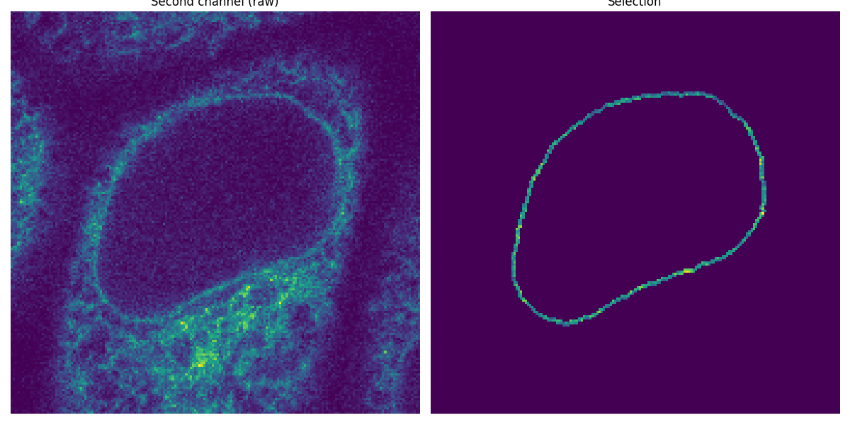
セグメント化された縁をマスクとして適用

最初のチャネルで核膜をセグメント化したので、それをマスクとして使用して、2番目のチャネルの強度を測定します。

image_t_0_channel_1 = image_sequence[0, 1, :, :]
selection = np.where(mask, image_t_0_channel_1, 0)

fig, (ax0, ax1) = plt.subplots(1, 2, figsize=(12, 6), sharey=True)

ax0.imshow(image_t_0_channel_1)
ax0.set_title('Second channel (raw)')
ax0.set_axis_off()

ax1.imshow(selection)
ax1.set_title('Selection')
ax1.set_axis_off()

fig.tight_layout()

総強度を測定

平均強度は、ラベル付き画像の領域プロパティとしてすぐに利用できます。

props = measure.regionprops_table(
    mask.astype(np.uint8),
    intensity_image=image_t_0_channel_1,
    properties=('label', 'area', 'intensity_mean'),
)

総強度の値を確認したい場合があります。

selection.sum()

np.uint64(28350)

から回復できることを確認したい場合があります。

props['area'] * props['intensity_mean']

array([28350.])

画像シーケンス全体の処理

時間点ごとにワークフローを反復する代わりに、（閾値処理ステップを除いて）多次元データセットを直接処理します。実際、ほとんどのscikit-image関数はnD画像をサポートしています。

n_z = image_sequence.shape[0]  # number of frames

smooth_seq = filters.gaussian(image_sequence[:, 0, :, :], sigma=(0, 1.5, 1.5))
thresh_values = [filters.threshold_otsu(s) for s in smooth_seq[:]]
thresh_seq = [smooth_seq[k, ...] > val for k, val in enumerate(thresh_values)]

あるいは、リスト内包表記を使用せずに、smooth_seqを2Dにする（最初の次元は時間点に対応し、2番目と最後の次元にはすべてのピクセル値が含まれる）ことでthresh_valuesを計算し、2番目の軸に沿って画像シーケンスに閾値処理関数を適用することもできます。

thresh_values = np.apply_along_axis(filters.threshold_otsu,
                                    axis=1,
                                    arr=smooth_seq.reshape(n_z, -1))

モルフォロジー演算には、以下の平坦な構造要素を使用します（np.newaxisは、時間の次元を追加するためにサイズ1の軸を先頭に追加します）。

footprint = ndi.generate_binary_structure(2, 1)[np.newaxis, ...]
footprint

array([[[False,  True, False],
        [ True,  True,  True],
        [False,  True, False]]])

これにより、各フレームは独立して処理されます（連続するフレームのピクセルが空間的に隣接することはありません）。

fill_seq = ndi.binary_fill_holes(thresh_seq, structure=footprint)

画像の境界に接するオブジェクトをクリアする際、一番下（最初）のフレームと一番上（最後）のフレームを境界として扱わないようにする必要があります。この場合、関連のある境界は、最大（x, y）値の端のみです。これは、以下のコードを実行することで3Dで確認できます。

import plotly.graph_objects as go

sample = fill_seq
(n_Z, n_Y, n_X) = sample.shape
Z, Y, X = np.mgrid[:n_Z, :n_Y, :n_X]

fig = go.Figure(
    data=go.Volume(
        x=X.flatten(),
        y=Y.flatten(),
        z=Z.flatten(),
        value=sample.flatten(),
        opacity=0.5,
        slices_z=dict(show=True, locations=[n_z // 2])
    )
)
fig.show()

border_mask = np.ones_like(fill_seq)
border_mask[n_z // 2, -1, -1] = False
clear_seq = segmentation.clear_border(fill_seq, mask=border_mask)

dilate_seq = morphology.binary_dilation(clear_seq, footprint=footprint)
erode_seq = morphology.binary_erosion(clear_seq, footprint=footprint)
mask_sequence = np.logical_and(dilate_seq, ~erode_seq)

各マスク（各時間点に対応）に、1から15までの異なるラベルを付けます。np.min_scalar_typeを使用して、時間点の数を表現するために必要な最小サイズの整数dtypeを決定します。

label_dtype = np.min_scalar_type(n_z)
mask_sequence = mask_sequence.astype(label_dtype)
labels = np.arange(1, n_z + 1, dtype=label_dtype)
mask_sequence *= labels[:, np.newaxis, np.newaxis]

これらのラベル付き領域すべてについて、関心のある領域プロパティを計算しましょう。

props = measure.regionprops_table(
    mask_sequence,
    intensity_image=image_sequence[:, 1, :, :],
    properties=('label', 'area', 'intensity_mean'),
)
np.testing.assert_array_equal(props['label'], np.arange(n_z) + 1)

fluorescence_change = [
    props['area'][i] * props['intensity_mean'][i] for i in range(n_z)
]

fluorescence_change /= fluorescence_change[0]  # normalization

fig, ax = plt.subplots()
ax.plot(fluorescence_change, 'rs')
ax.grid()
ax.set_xlabel('Time point')
ax.set_ylabel('Normalized total intensity')
ax.set_title('Change in fluorescence intensity at the nuclear envelope')
fig.tight_layout()

plt.show()

予想どおりの結果が得られました。核膜での総蛍光強度は、最初の5つの時間点で1.3倍増加し、その後ほぼ一定になります。