円形および楕円形ハフ変換

最も単純な形式のハフ変換は、直線を検出する方法ですが、円や楕円を検出するためにも使用できます。アルゴリズムはエッジが検出されていることを前提としており、ノイズや欠落点に対してロバストです。

円検出

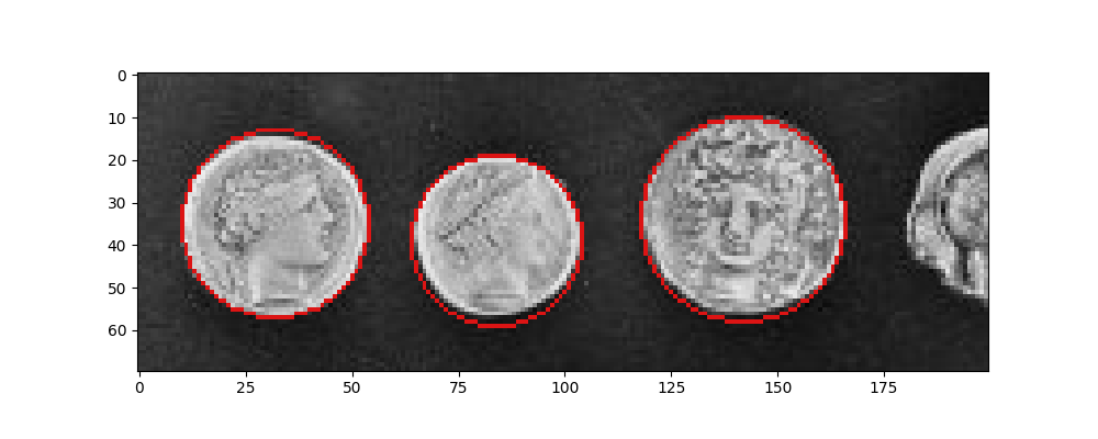
次の例では、ハフ変換を使用してコインの位置を検出し、それらのエッジを一致させます。考えられる半径の範囲を指定します。各半径について、2つの円が抽出され、最終的に最も顕著な5つの候補を保持します。結果は、コインの位置が適切に検出されていることを示しています。

アルゴリズムの概要

白い背景に黒い円がある場合、最初にその半径（または半径の範囲）を推測して新しい円を構築します。この円は元の画像の各黒ピクセルに適用され、この円の座標はアキュムレータで投票されます。この幾何学的構成から、元の円の中心位置が最高のスコアを受け取ります。

アキュムレータのサイズは、フレーム外のセンターを検出するために、元の画像よりも大きく構築されていることに注意してください。そのサイズは、より大きな半径の2倍に拡張されます。

import numpy as np
import matplotlib.pyplot as plt

from skimage import data, color
from skimage.transform import hough_circle, hough_circle_peaks
from skimage.feature import canny
from skimage.draw import circle_perimeter
from skimage.util import img_as_ubyte


# Load picture and detect edges
image = img_as_ubyte(data.coins()[160:230, 70:270])
edges = canny(image, sigma=3, low_threshold=10, high_threshold=50)


# Detect two radii
hough_radii = np.arange(20, 35, 2)
hough_res = hough_circle(edges, hough_radii)

# Select the most prominent 3 circles
accums, cx, cy, radii = hough_circle_peaks(hough_res, hough_radii, total_num_peaks=3)

# Draw them
fig, ax = plt.subplots(ncols=1, nrows=1, figsize=(10, 4))
image = color.gray2rgb(image)
for center_y, center_x, radius in zip(cy, cx, radii):
    circy, circx = circle_perimeter(center_y, center_x, radius, shape=image.shape)
    image[circy, circx] = (220, 20, 20)

ax.imshow(image, cmap=plt.cm.gray)
plt.show()

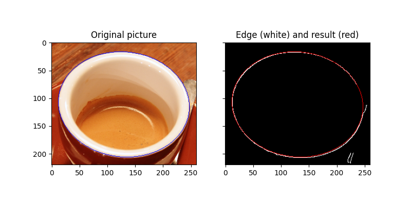
楕円検出

この2番目の例では、コーヒーカップの縁を検出することを目的としています。基本的には、これは円の投影、つまり楕円です。解決すべき問題は、円の場合は3つではなく、5つのパラメータを決定する必要があるため、はるかに困難です。

アルゴリズムの概要

アルゴリズムは、楕円に属する2つの異なる点を取ります。これらの2つの点が長軸を形成すると仮定します。他のすべての点のループは、候補楕円の短軸の長さを決定します。後者は、十分な数の「有効な」候補が同様の短軸の長さを持っている場合、結果に含まれます。有効とは、短軸と長軸の長さが所定の範囲内にある候補を意味します。アルゴリズムの完全な説明は、参考文献[1]にあります。

参考文献

[1]

Xie、Yonghong、およびQiang Ji。「新しい効率的な楕円検出方法。」パターン認識、2002年。議事録。第16回国際会議。Vol。2. IEEE、2002年

import matplotlib.pyplot as plt

from skimage import data, color, img_as_ubyte
from skimage.feature import canny
from skimage.transform import hough_ellipse
from skimage.draw import ellipse_perimeter

# Load picture, convert to grayscale and detect edges
image_rgb = data.coffee()[0:220, 160:420]
image_gray = color.rgb2gray(image_rgb)
edges = canny(image_gray, sigma=2.0, low_threshold=0.55, high_threshold=0.8)

# Perform a Hough Transform
# The accuracy corresponds to the bin size of the histogram for minor axis lengths.
# A higher `accuracy` value will lead to more ellipses being found, at the
# cost of a lower precision on the minor axis length estimation.
# A higher `threshold` will lead to less ellipses being found, filtering out those
# with fewer edge points (as found above by the Canny detector) on their perimeter.
result = hough_ellipse(edges, accuracy=20, threshold=250, min_size=100, max_size=120)
result.sort(order='accumulator')

# Estimated parameters for the ellipse
best = list(result[-1])
yc, xc, a, b = (int(round(x)) for x in best[1:5])
orientation = best[5]

# Draw the ellipse on the original image
cy, cx = ellipse_perimeter(yc, xc, a, b, orientation)
image_rgb[cy, cx] = (0, 0, 255)
# Draw the edge (white) and the resulting ellipse (red)
edges = color.gray2rgb(img_as_ubyte(edges))
edges[cy, cx] = (250, 0, 0)

fig2, (ax1, ax2) = plt.subplots(
    ncols=2, nrows=1, figsize=(8, 4), sharex=True, sharey=True
)

ax1.set_title('Original picture')
ax1.imshow(image_rgb)

ax2.set_title('Edge (white) and result (red)')
ax2.imshow(edges)

plt.show()