位相アンラップ#

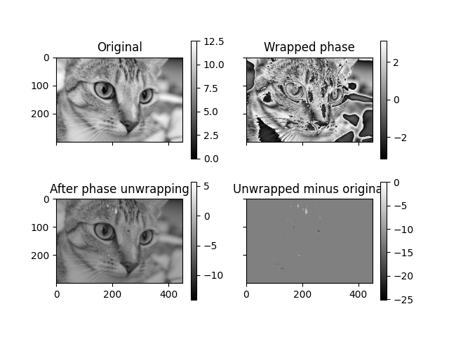
一部の信号は2*piを法としてのみ観測でき、これは2次元および3次元の画像にも適用できます。これらの場合、位相アンラップは、基礎となるアンラップされた信号を復元するために必要です。この例では、このような問題に対してskimageに実装されているアルゴリズム[1]をデモンストレーションします。1次元、2次元、3次元の画像はすべてskimageを使用してアンラップできます。ここでは、2次元の場合の位相アンラップをデモンストレーションします。

import numpy as np
from matplotlib import pyplot as plt
from skimage import data, img_as_float, color, exposure
from skimage.restoration import unwrap_phase


# Load an image as a floating-point grayscale
image = color.rgb2gray(img_as_float(data.chelsea()))
# Scale the image to [0, 4*pi]
image = exposure.rescale_intensity(image, out_range=(0, 4 * np.pi))
# Create a phase-wrapped image in the interval [-pi, pi)
image_wrapped = np.angle(np.exp(1j * image))
# Perform phase unwrapping
image_unwrapped = unwrap_phase(image_wrapped)

fig, ax = plt.subplots(2, 2, sharex=True, sharey=True)
ax1, ax2, ax3, ax4 = ax.ravel()

fig.colorbar(ax1.imshow(image, cmap='gray', vmin=0, vmax=4 * np.pi), ax=ax1)
ax1.set_title('Original')

fig.colorbar(ax2.imshow(image_wrapped, cmap='gray', vmin=-np.pi, vmax=np.pi), ax=ax2)
ax2.set_title('Wrapped phase')

fig.colorbar(ax3.imshow(image_unwrapped, cmap='gray'), ax=ax3)
ax3.set_title('After phase unwrapping')

fig.colorbar(ax4.imshow(image_unwrapped - image, cmap='gray'), ax=ax4)
ax4.set_title('Unwrapped minus original')

Original, Wrapped phase, After phase unwrapping, Unwrapped minus original

Text(0.5, 1.0, 'Unwrapped minus original')

アンラップ手順はマスクされた配列を受け入れ、オプションで画像の端を接続するために循環境界を想定することもできます。以下の例では、画像の行をマスクすることによって2つに分割された単純な位相ランプを調べます。

# Create a simple ramp
image = np.ones((100, 100)) * np.linspace(0, 8 * np.pi, 100).reshape((-1, 1))
# Mask the image to split it in two horizontally
mask = np.zeros_like(image, dtype=bool)
mask[image.shape[0] // 2, :] = True

image_wrapped = np.ma.array(np.angle(np.exp(1j * image)), mask=mask)
# Unwrap image without wrap around
image_unwrapped_no_wrap_around = unwrap_phase(image_wrapped, wrap_around=(False, False))
# Unwrap with wrap around enabled for the 0th dimension
image_unwrapped_wrap_around = unwrap_phase(image_wrapped, wrap_around=(True, False))

fig, ax = plt.subplots(2, 2)
ax1, ax2, ax3, ax4 = ax.ravel()

fig.colorbar(ax1.imshow(np.ma.array(image, mask=mask), cmap='rainbow'), ax=ax1)
ax1.set_title('Original')

fig.colorbar(ax2.imshow(image_wrapped, cmap='rainbow', vmin=-np.pi, vmax=np.pi), ax=ax2)
ax2.set_title('Wrapped phase')

fig.colorbar(ax3.imshow(image_unwrapped_no_wrap_around, cmap='rainbow'), ax=ax3)
ax3.set_title('Unwrapped without wrap_around')

fig.colorbar(ax4.imshow(image_unwrapped_wrap_around, cmap='rainbow'), ax=ax4)
ax4.set_title('Unwrapped with wrap_around')

plt.tight_layout()
plt.show()

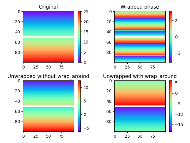
Original, Wrapped phase, Unwrapped without wrap_around, Unwrapped with wrap_around

上の図では、マスクされた行は画像全体にわたる白い線として見ることができます。下の行にある2つのアンラップされた画像の違いは明らかです。（左下の）アンラップなしの場合、マスクされた境界の上下の領域はまったく相互作用せず、結果として2つの領域間に任意の整数倍の2piのオフセットが生じます。領域を2つの別々の画像としてアンラップすることもできました。（右下の）垂直方向にラップアラウンドを有効にすると、状況が変わります。アンラップパスが画像の下部から上部、またはその逆に移動できるようになり、事実上、2つの領域間のオフセットを決定する方法が提供されます。

参考文献#

スクリプトの総実行時間： (0分1.315秒)

Sphinx-Galleryによって生成されたギャラリー