形状指数

形状指数は、Koenderink & van Doorn [1] によって定義された、ヘッセ行列の固有値から導出される、局所曲率の単一値尺度です。

これは、見かけの局所形状に基づいて構造を見つけるために使用できます。

形状指数は、-1から1までの値にマッピングされ、異なる種類の形状を表します（詳細はドキュメントを参照）。

この例では、検出する必要のあるスポットを持つランダムな画像が生成されます。

形状指数1は、「球形キャップ」、つまり検出したいスポットの形状を表します。

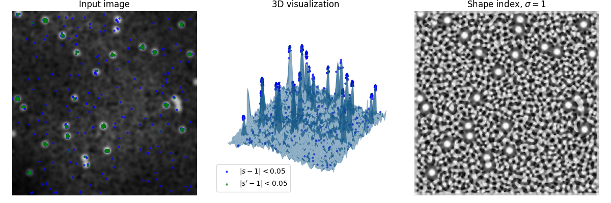
左端のプロットは生成された画像を示し、中央は強度値を3Dサーフェスの高さとして使用した画像の3Dレンダリングを示し、右端は形状指数（s）を示します。

見てわかるように、形状指数はノイズの局所形状も容易に増幅しますが、グローバルな現象（例：不均一な照明）の影響を受けません。

青と緑のマークは、目的の形状から0.05以下しか逸脱しない点です。信号のノイズを減衰させるために、緑のマークは、別のガウスぼかしパス（s'を生成）後の形状指数（s）から取得されます。

近すぎるスポットは、目的の形状を持っていないため、検出*されない*ことに注意してください。

[1]

Koenderink, J. J. & van Doorn, A. J., “Surface shape and curvature scales”, Image and Vision Computing, 1992, 10, 557-564. DOI:10.1016/0262-8856(92)90076-F

import numpy as np
import matplotlib.pyplot as plt
from scipy import ndimage as ndi
from skimage.feature import shape_index
from skimage.draw import disk


def create_test_image(image_size=256, spot_count=30, spot_radius=5, cloud_noise_size=4):
    """
    Generate a test image with random noise, uneven illumination and spots.
    """
    rng = np.random.default_rng()
    image = rng.normal(loc=0.25, scale=0.25, size=(image_size, image_size))

    for _ in range(spot_count):
        rr, cc = disk(
            (rng.integers(image.shape[0]), rng.integers(image.shape[1])),
            spot_radius,
            shape=image.shape,
        )
        image[rr, cc] = 1

    image *= rng.normal(loc=1.0, scale=0.1, size=image.shape)

    image *= ndi.zoom(
        rng.normal(loc=1.0, scale=0.5, size=(cloud_noise_size, cloud_noise_size)),
        image_size / cloud_noise_size,
    )

    return ndi.gaussian_filter(image, sigma=2.0)


# First create the test image and its shape index

image = create_test_image()

s = shape_index(image)

# In this example we want to detect 'spherical caps',
# so we threshold the shape index map to
# find points which are 'spherical caps' (~1)

target = 1
delta = 0.05

point_y, point_x = np.where(np.abs(s - target) < delta)
point_z = image[point_y, point_x]

# The shape index map relentlessly produces the shape, even that of noise.
# In order to reduce the impact of noise, we apply a Gaussian filter to it,
# and show the results once in

s_smooth = ndi.gaussian_filter(s, sigma=0.5)

point_y_s, point_x_s = np.where(np.abs(s_smooth - target) < delta)
point_z_s = image[point_y_s, point_x_s]


fig = plt.figure(figsize=(12, 4))
ax1 = fig.add_subplot(1, 3, 1)

ax1.imshow(image, cmap=plt.cm.gray)
ax1.axis('off')
ax1.set_title('Input image')

scatter_settings = dict(alpha=0.75, s=10, linewidths=0)

ax1.scatter(point_x, point_y, color='blue', **scatter_settings)
ax1.scatter(point_x_s, point_y_s, color='green', **scatter_settings)

ax2 = fig.add_subplot(1, 3, 2, projection='3d', sharex=ax1, sharey=ax1)

x, y = np.meshgrid(np.arange(0, image.shape[0], 1), np.arange(0, image.shape[1], 1))

ax2.plot_surface(x, y, image, linewidth=0, alpha=0.5)

ax2.scatter(
    point_x, point_y, point_z, color='blue', label='$|s - 1|<0.05$', **scatter_settings
)

ax2.scatter(
    point_x_s,
    point_y_s,
    point_z_s,
    color='green',
    label='$|s\' - 1|<0.05$',
    **scatter_settings,
)

ax2.legend(loc='lower left')

ax2.axis('off')
ax2.set_title('3D visualization')

ax3 = fig.add_subplot(1, 3, 3, sharex=ax1, sharey=ax1)

ax3.imshow(s, cmap=plt.cm.gray)
ax3.axis('off')
ax3.set_title(r'Shape index, $\sigma=1$')

fig.tight_layout()

plt.show()