GLCMテクスチャ特徴

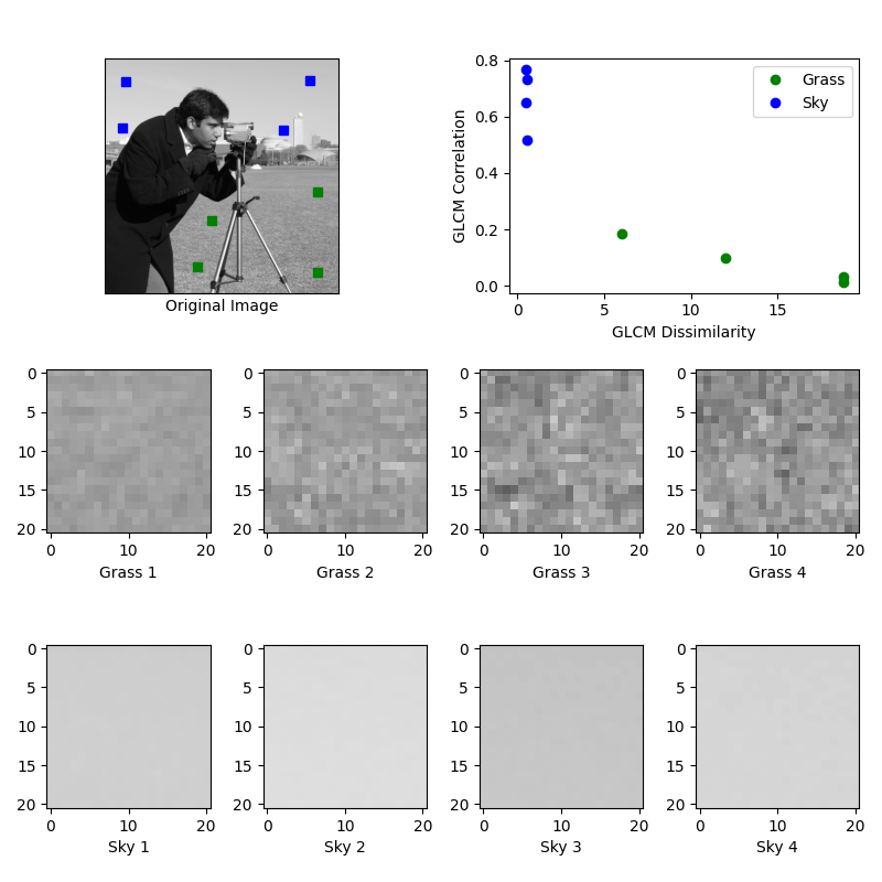
この例では、グレイレベル同時生起行列（GLCM）[1]を用いたテクスチャ分類について説明します。GLCMは、画像上の特定のオフセットにおける同時生起するグレースケール値のヒストグラムです。

この例では、画像から2種類のテクスチャのサンプル（草地と空の領域）を抽出します。各パッチについて、5の水平オフセット（distance=[5]およびangles=[0]）を持つGLCMを計算します。次に、GLCM行列の2つの特徴、非類似度と相関を計算します。これらをプロットして、クラスが特徴空間でクラスタを形成することを示します。典型的な分類問題では、最後のステップ（この例には含まれていません）は、ロジスティック回帰などの分類器をトレーニングして、新しい画像から画像パッチにラベルを付けることです。

バージョン0.19で変更されました: greymatrixは0.19でgraymatrixに名前変更されました。

バージョン0.19で変更されました: greycopropsは0.19でgraycopropsに名前変更されました。

参考文献

[1]

Haralick, RM.; Shanmugam, K., “画像分類のためのテクスチャ特徴” IEEE Transactions on systems, man, and cybernetics 6 (1973): 610-621. DOI:10.1109/TSMC.1973.4309314

import matplotlib.pyplot as plt

from skimage.feature import graycomatrix, graycoprops
from skimage import data


PATCH_SIZE = 21

# open the camera image
image = data.camera()

# select some patches from grassy areas of the image
grass_locations = [(280, 454), (342, 223), (444, 192), (455, 455)]
grass_patches = []
for loc in grass_locations:
    grass_patches.append(
        image[loc[0] : loc[0] + PATCH_SIZE, loc[1] : loc[1] + PATCH_SIZE]
    )

# select some patches from sky areas of the image
sky_locations = [(38, 34), (139, 28), (37, 437), (145, 379)]
sky_patches = []
for loc in sky_locations:
    sky_patches.append(
        image[loc[0] : loc[0] + PATCH_SIZE, loc[1] : loc[1] + PATCH_SIZE]
    )

# compute some GLCM properties each patch
xs = []
ys = []
for patch in grass_patches + sky_patches:
    glcm = graycomatrix(
        patch, distances=[5], angles=[0], levels=256, symmetric=True, normed=True
    )
    xs.append(graycoprops(glcm, 'dissimilarity')[0, 0])
    ys.append(graycoprops(glcm, 'correlation')[0, 0])

# create the figure
fig = plt.figure(figsize=(8, 8))

# display original image with locations of patches
ax = fig.add_subplot(3, 2, 1)
ax.imshow(image, cmap=plt.cm.gray, vmin=0, vmax=255)
for y, x in grass_locations:
    ax.plot(x + PATCH_SIZE / 2, y + PATCH_SIZE / 2, 'gs')
for y, x in sky_locations:
    ax.plot(x + PATCH_SIZE / 2, y + PATCH_SIZE / 2, 'bs')
ax.set_xlabel('Original Image')
ax.set_xticks([])
ax.set_yticks([])
ax.axis('image')

# for each patch, plot (dissimilarity, correlation)
ax = fig.add_subplot(3, 2, 2)
ax.plot(xs[: len(grass_patches)], ys[: len(grass_patches)], 'go', label='Grass')
ax.plot(xs[len(grass_patches) :], ys[len(grass_patches) :], 'bo', label='Sky')
ax.set_xlabel('GLCM Dissimilarity')
ax.set_ylabel('GLCM Correlation')
ax.legend()

# display the image patches
for i, patch in enumerate(grass_patches):
    ax = fig.add_subplot(3, len(grass_patches), len(grass_patches) * 1 + i + 1)
    ax.imshow(patch, cmap=plt.cm.gray, vmin=0, vmax=255)
    ax.set_xlabel(f"Grass {i + 1}")

for i, patch in enumerate(sky_patches):
    ax = fig.add_subplot(3, len(sky_patches), len(sky_patches) * 2 + i + 1)
    ax.imshow(patch, cmap=plt.cm.gray, vmin=0, vmax=255)
    ax.set_xlabel(f"Sky {i + 1}")


# display the patches and plot
fig.suptitle('Grey level co-occurrence matrix features', fontsize=14, y=1.05)
plt.tight_layout()
plt.show()