Haar-like特徴記述子を用いた顔分類

Haar-like特徴記述子は、最初のリアルタイム顔検出器を実装するために成功裏に使用されました [1]。このアプリケーションに触発されて、顔と非顔を検出するためのHaar-like特徴の抽出、選択、および分類を示す例を提案します。

注意

この例は、特徴選択と分類のためにscikit-learnに依存しています。

参考文献

[1]

Viola, Paul, and Michael J. Jones. “Robust real-time face detection.” International journal of computer vision 57.2 (2004): 137-154. https://www.merl.com/publications/docs/TR2004-043.pdf DOI:10.1109/CVPR.2001.990517

from time import time

import numpy as np
import matplotlib.pyplot as plt

from sklearn.ensemble import RandomForestClassifier
from sklearn.model_selection import train_test_split
from sklearn.metrics import roc_auc_score

from skimage.data import lfw_subset
from skimage.transform import integral_image
from skimage.feature import haar_like_feature
from skimage.feature import haar_like_feature_coord
from skimage.feature import draw_haar_like_feature

画像からHaar-like特徴を抽出する手順は比較的簡単です。まず、関心領域（ROI）を定義します。次に、このROI内の積分画像を計算します。最後に、積分画像を使用して特徴を抽出します。

def extract_feature_image(img, feature_type, feature_coord=None):
    """Extract the haar feature for the current image"""
    ii = integral_image(img)
    return haar_like_feature(
        ii,
        0,
        0,
        ii.shape[0],
        ii.shape[1],
        feature_type=feature_type,
        feature_coord=feature_coord,
    )

100枚の顔画像と100枚の非顔画像で構成されるCBCLデータセットのサブセットを使用します。各画像は、19x19ピクセルのROIにリサイズされています。分類器をトレーニングし、最も顕著な特徴を決定するために、各グループから75枚の画像を選択します。各クラスの残りの25枚の画像は、分類器のパフォーマンスを評価するために使用されます。

images = lfw_subset()
# To speed up the example, extract the two types of features only
feature_types = ['type-2-x', 'type-2-y']

# Compute the result
t_start = time()
X = [extract_feature_image(img, feature_types) for img in images]
X = np.stack(X)
time_full_feature_comp = time() - t_start

# Label images (100 faces and 100 non-faces)
y = np.array([1] * 100 + [0] * 100)

X_train, X_test, y_train, y_test = train_test_split(
    X, y, train_size=150, random_state=0, stratify=y
)

# Extract all possible features
feature_coord, feature_type = haar_like_feature_coord(
    width=images.shape[2], height=images.shape[1], feature_type=feature_types
)

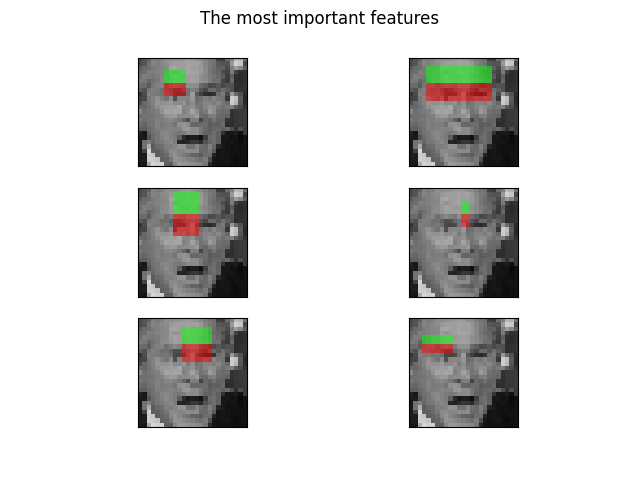
ランダムフォレスト分類器は、特に顔分類のために、最も顕著な特徴を選択するためにトレーニングできます。このアイデアは、木のアンサンブルによって最も頻繁に使用される特徴を決定することです。後続のステップで最も顕著な特徴のみを使用することにより、精度を維持しながら計算を大幅に高速化できます。

# Train a random forest classifier and assess its performance
clf = RandomForestClassifier(
    n_estimators=1000, max_depth=None, max_features=100, n_jobs=-1, random_state=0
)
t_start = time()
clf.fit(X_train, y_train)
time_full_train = time() - t_start
auc_full_features = roc_auc_score(y_test, clf.predict_proba(X_test)[:, 1])

# Sort features in order of importance and plot the six most significant
idx_sorted = np.argsort(clf.feature_importances_)[::-1]

fig, axes = plt.subplots(3, 2)
for idx, ax in enumerate(axes.ravel()):
    image = images[0]
    image = draw_haar_like_feature(
        image, 0, 0, images.shape[2], images.shape[1], [feature_coord[idx_sorted[idx]]]
    )
    ax.imshow(image)
    ax.set_xticks([])
    ax.set_yticks([])

_ = fig.suptitle('The most important features')

特徴重要度の累積和を確認することで、最も重要な特徴を選択できます。この例では、累積値の70％を表す特徴を保持します（これは、特徴の総数のわずか3％を使用することに対応します）。

cdf_feature_importances = np.cumsum(clf.feature_importances_[idx_sorted])
cdf_feature_importances /= cdf_feature_importances[-1]  # divide by max value
sig_feature_count = np.count_nonzero(cdf_feature_importances < 0.7)
sig_feature_percent = round(sig_feature_count / len(cdf_feature_importances) * 100, 1)
print(
    f'{sig_feature_count} features, or {sig_feature_percent}%, '
    f'account for 70% of branch points in the random forest.'
)

# Select the determined number of most informative features
feature_coord_sel = feature_coord[idx_sorted[:sig_feature_count]]
feature_type_sel = feature_type[idx_sorted[:sig_feature_count]]
# Note: it is also possible to select the features directly from the matrix X,
# but we would like to emphasize the usage of `feature_coord` and `feature_type`
# to recompute a subset of desired features.

# Compute the result
t_start = time()
X = [extract_feature_image(img, feature_type_sel, feature_coord_sel) for img in images]
X = np.stack(X)
time_subs_feature_comp = time() - t_start

y = np.array([1] * 100 + [0] * 100)
X_train, X_test, y_train, y_test = train_test_split(
    X, y, train_size=150, random_state=0, stratify=y
)

712 features, or 0.7%, account for 70% of branch points in the random forest.

特徴が抽出されたら、新しい分類器をトレーニングおよびテストできます。

t_start = time()
clf.fit(X_train, y_train)
time_subs_train = time() - t_start

auc_subs_features = roc_auc_score(y_test, clf.predict_proba(X_test)[:, 1])

summary = (
    f'Computing the full feature set took '
    f'{time_full_feature_comp:.3f}s, '
    f'plus {time_full_train:.3f}s training, '
    f'for an AUC of {auc_full_features:.2f}. '
    f'Computing the restricted feature set took '
    f'{time_subs_feature_comp:.3f}s, plus {time_subs_train:.3f}s '
    f'training, for an AUC of {auc_subs_features:.2f}.'
)

print(summary)
plt.show()

Computing the full feature set took 29.998s, plus 3.076s training, for an AUC of 1.00. Computing the restricted feature set took 0.170s, plus 2.463s training, for an AUC of 1.00.