ローカル特徴量とランダムフォレストを用いた訓練可能なセグメンテーション

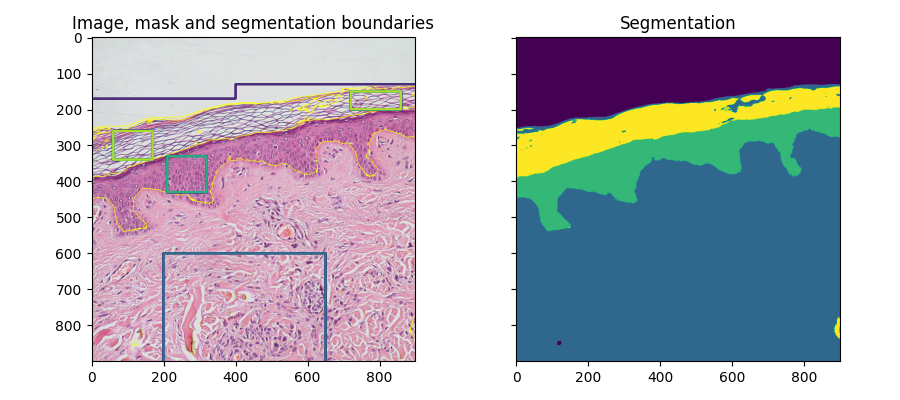
ここでは、異なるスケールでの局所強度、エッジ、テクスチャに基づくローカル特徴量を用いて、ピクセルベースのセグメンテーションが計算されます。ユーザーが提供するマスクを使用して、異なる領域が識別されます。マスクのピクセルは、scikit-learnのランダムフォレスト分類器 [1] を訓練するために使用されます。ラベルのないピクセルは、分類器の予測からラベル付けされます。

このセグメンテーションアルゴリズムは、ilastik [2] やImageJ [3] などの他のソフトウェアでは、訓練可能なセグメンテーションと呼ばれています（「wekaセグメンテーション」とも呼ばれます）。

[1]

https://scikit-learn.org/stable/modules/generated/sklearn.ensemble.RandomForestClassifier.html

[2]

https://www.ilastik.org/documentation/pixelclassification/pixelclassification

[3]

https://imagej.net/Trainable_Weka_Segmentation#Training_features_.282D.29

import numpy as np
import matplotlib.pyplot as plt
from skimage import data, segmentation, feature, future
from sklearn.ensemble import RandomForestClassifier
from functools import partial

full_img = data.skin()

img = full_img[:900, :900]

# Build an array of labels for training the segmentation.
# Here we use rectangles but visualization libraries such as plotly
# (and napari?) can be used to draw a mask on the image.
training_labels = np.zeros(img.shape[:2], dtype=np.uint8)
training_labels[:130] = 1
training_labels[:170, :400] = 1
training_labels[600:900, 200:650] = 2
training_labels[330:430, 210:320] = 3
training_labels[260:340, 60:170] = 4
training_labels[150:200, 720:860] = 4

sigma_min = 1
sigma_max = 16
features_func = partial(
    feature.multiscale_basic_features,
    intensity=True,
    edges=False,
    texture=True,
    sigma_min=sigma_min,
    sigma_max=sigma_max,
    channel_axis=-1,
)
features = features_func(img)
clf = RandomForestClassifier(n_estimators=50, n_jobs=-1, max_depth=10, max_samples=0.05)
clf = future.fit_segmenter(training_labels, features, clf)
result = future.predict_segmenter(features, clf)

fig, ax = plt.subplots(1, 2, sharex=True, sharey=True, figsize=(9, 4))
ax[0].imshow(segmentation.mark_boundaries(img, result, mode='thick'))
ax[0].contour(training_labels)
ax[0].set_title('Image, mask and segmentation boundaries')
ax[1].imshow(result)
ax[1].set_title('Segmentation')
fig.tight_layout()

特徴量の重要度

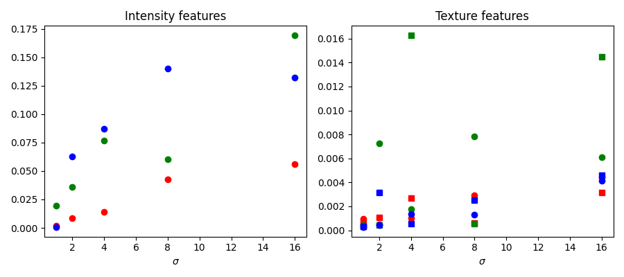
以下では、scikit-learnによって計算された、異なる特徴量の重要度を調べます。強度の特徴量は、テクスチャの特徴量よりもはるかに重要度が高くなっています。計算時間を短縮するために、この情報を使用して分類器に与える特徴量の数を減らしたくなるかもしれません。ただし、これは過剰適合につながり、領域間の境界で結果が悪化する可能性があります。

fig, ax = plt.subplots(1, 2, figsize=(9, 4))
l = len(clf.feature_importances_)
feature_importance = (
    clf.feature_importances_[: l // 3],
    clf.feature_importances_[l // 3 : 2 * l // 3],
    clf.feature_importances_[2 * l // 3 :],
)
sigmas = np.logspace(
    np.log2(sigma_min),
    np.log2(sigma_max),
    num=int(np.log2(sigma_max) - np.log2(sigma_min) + 1),
    base=2,
    endpoint=True,
)
for ch, color in zip(range(3), ['r', 'g', 'b']):
    ax[0].plot(sigmas, feature_importance[ch][::3], 'o', color=color)
    ax[0].set_title("Intensity features")
    ax[0].set_xlabel("$\\sigma$")
for ch, color in zip(range(3), ['r', 'g', 'b']):
    ax[1].plot(sigmas, feature_importance[ch][1::3], 'o', color=color)
    ax[1].plot(sigmas, feature_importance[ch][2::3], 's', color=color)
    ax[1].set_title("Texture features")
    ax[1].set_xlabel("$\\sigma$")

fig.tight_layout()

新しい画像のフィッティング

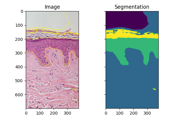
同様の条件で取得された同様のオブジェクトの画像が複数ある場合、fit_segmenterで訓練された分類器を使用して他の画像をセグメント化できます。以下の例では、画像の別の部分を使用しています。

img_new = full_img[:700, 900:]

features_new = features_func(img_new)
result_new = future.predict_segmenter(features_new, clf)
fig, ax = plt.subplots(1, 2, sharex=True, sharey=True, figsize=(6, 4))
ax[0].imshow(segmentation.mark_boundaries(img_new, result_new, mode='thick'))
ax[0].set_title('Image')
ax[1].imshow(result_new)
ax[1].set_title('Segmentation')
fig.tight_layout()

plt.show()