Max-tree

Max-treeは、多数の形態学的フィルタの基礎となる画像の階層的表現です。

画像に閾値処理を適用すると、1つ以上の連結成分を含む2値画像が得られます。より低い閾値を適用すると、より高い閾値からのすべての連結成分は、より低い閾値からの連結成分に含まれます。これは、木で表現できる入れ子の成分の階層を自然に定義します。閾値t1で閾値処理によって得られた連結成分Aが、閾値t1 < t2で閾値処理によって得られた成分Bに含まれる場合、BはAの親であると言います。得られた木構造はコンポーネントツリーと呼ばれ、Max-treeはこのようなコンポーネントツリーのコンパクトな表現です。[1]、[2]、[3]、[4]

この例では、Max-treeの概要を示します。

参考文献

[1]

Salembier, P., Oliveras, A., & Garrido, L. (1998). Antiextensive Connected Operators for Image and Sequence Processing. IEEE Transactions on Image Processing, 7(4), 555-570. DOI:10.1109/83.663500

[2]

Berger, C., Geraud, T., Levillain, R., Widynski, N., Baillard, A., Bertin, E. (2007). Effective Component Tree Computation with Application to Pattern Recognition in Astronomical Imaging. In International Conference on Image Processing (ICIP) (pp. 41-44). DOI:10.1109/ICIP.2007.4379949

[3]

Najman, L., & Couprie, M. (2006). Building the component tree in quasi-linear time. IEEE Transactions on Image Processing, 15(11), 3531-3539. DOI:10.1109/TIP.2006.877518

[4]

Carlinet, E., & Geraud, T. (2014). A Comparative Review of Component Tree Computation Algorithms. IEEE Transactions on Image Processing, 23(9), 3885-3895. DOI:10.1109/TIP.2014.2336551

import numpy as np
import matplotlib.pyplot as plt
from matplotlib.lines import Line2D
from skimage.morphology import max_tree
import networkx as nx

始める前に：いくつかのヘルパー関数

def plot_img(ax, image, title, plot_text, image_values):
    """Plot an image, overlaying image values or indices."""
    ax.imshow(image, cmap='gray', aspect='equal', vmin=0, vmax=np.max(image))
    ax.set_title(title)
    ax.set_yticks([])
    ax.set_xticks([])

    for x in np.arange(-0.5, image.shape[0], 1.0):
        ax.add_artist(
            Line2D((x, x), (-0.5, image.shape[0] - 0.5), color='blue', linewidth=2)
        )

    for y in np.arange(-0.5, image.shape[1], 1.0):
        ax.add_artist(Line2D((-0.5, image.shape[1]), (y, y), color='blue', linewidth=2))

    if plot_text:
        for i, j in np.ndindex(*image_values.shape):
            ax.text(
                j,
                i,
                image_values[i, j],
                fontsize=8,
                horizontalalignment='center',
                verticalalignment='center',
                color='red',
            )
    return


def prune(G, node, res):
    """Transform a canonical max tree to a max tree."""
    value = G.nodes[node]['value']
    res[node] = str(node)
    preds = [p for p in G.predecessors(node)]
    for p in preds:
        if G.nodes[p]['value'] == value:
            res[node] += f", {p}"
            G.remove_node(p)
        else:
            prune(G, p, res)
    G.nodes[node]['label'] = res[node]
    return


def accumulate(G, node, res):
    """Transform a max tree to a component tree."""
    total = G.nodes[node]['label']
    parents = G.predecessors(node)
    for p in parents:
        total += ', ' + accumulate(G, p, res)
    res[node] = total
    return total


def position_nodes_for_max_tree(G, image_rav, root_x=4, delta_x=1.2):
    """Set the position of nodes of a max-tree.

    This function helps to visually distinguish between nodes at the same
    level of the hierarchy and nodes at different levels.
    """
    pos = {}
    for node in reversed(list(nx.topological_sort(canonical_max_tree))):
        value = G.nodes[node]['value']
        if canonical_max_tree.out_degree(node) == 0:
            # root
            pos[node] = (root_x, value)

        in_nodes = [y for y in canonical_max_tree.predecessors(node)]

        # place the nodes at the same level
        level_nodes = [y for y in filter(lambda x: image_rav[x] == value, in_nodes)]
        nb_level_nodes = len(level_nodes) + 1

        c = nb_level_nodes // 2
        i = -c
        if len(level_nodes) < 3:
            hy = 0
            m = 0
        else:
            hy = 0.25
            m = hy / (c - 1)

        for level_node in level_nodes:
            if i == 0:
                i += 1
            if len(level_nodes) < 3:
                pos[level_node] = (pos[node][0] + i * 0.6 * delta_x, value)
            else:
                pos[level_node] = (
                    pos[node][0] + i * 0.6 * delta_x,
                    value + m * (2 * np.abs(i) - c - 1),
                )
            i += 1

        # place the nodes at different levels
        other_level_nodes = [
            y for y in filter(lambda x: image_rav[x] > value, in_nodes)
        ]
        if len(other_level_nodes) == 1:
            i = 0
        else:
            i = -len(other_level_nodes) // 2
        for other_level_node in other_level_nodes:
            if (len(other_level_nodes) % 2 == 0) and (i == 0):
                i += 1
            pos[other_level_node] = (
                pos[node][0] + i * delta_x,
                image_rav[other_level_node],
            )
            i += 1

    return pos


def plot_tree(graph, positions, ax, *, title='', labels=None, font_size=8, text_size=8):
    """Plot max and component trees."""
    nx.draw_networkx(
        graph,
        pos=positions,
        ax=ax,
        node_size=40,
        node_shape='s',
        node_color='white',
        font_size=font_size,
        labels=labels,
    )
    for v in range(image_rav.min(), image_rav.max() + 1):
        ax.hlines(v - 0.5, -3, 10, linestyles='dotted')
        ax.text(-3, v - 0.15, f"val: {v}", fontsize=text_size)
    ax.hlines(v + 0.5, -3, 10, linestyles='dotted')
    ax.set_xlim(-3, 10)
    ax.set_title(title)
    ax.set_axis_off()

画像の定義

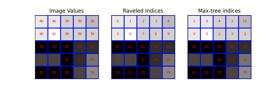
小さなテスト画像を定義します。明確にするために、画像値とインデックスを混同できない例として画像を選択します（異なる範囲）。

image = np.array(
    [
        [40, 40, 39, 39, 38],
        [40, 41, 39, 39, 39],
        [30, 30, 30, 32, 32],
        [33, 33, 30, 32, 35],
        [30, 30, 30, 33, 36],
    ],
    dtype=np.uint8,
)

Max-tree

次に、この画像のMax-treeを計算します。画像のMax-tree

P, S = max_tree(image)

P_rav = P.ravel()

画像のプロット

次に、画像とその展開されたインデックスを視覚化します。具体的には、次のオーバーレイを含む画像をプロットします： - 画像値 - 展開されたインデックス（ピクセル識別子として機能します） - max_tree関数の出力

# raveled image
image_rav = image.ravel()

# raveled indices of the example image (for display purpose)
raveled_indices = np.arange(image.size).reshape(image.shape)

fig, (ax1, ax2, ax3) = plt.subplots(1, 3, sharey=True, figsize=(9, 3))

plot_img(ax1, image - image.min(), 'Image Values', plot_text=True, image_values=image)
plot_img(
    ax2,
    image - image.min(),
    'Raveled Indices',
    plot_text=True,
    image_values=raveled_indices,
)
plot_img(ax3, image - image.min(), 'Max-tree indices', plot_text=True, image_values=P)

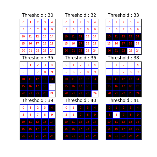
閾値処理の可視化

次に、一連の閾値処理の結果を調べます。コンポーネントツリー（およびMax-tree）は、異なるレベルでの連結成分間の包含関係の表現を提供します。

fig, axes = plt.subplots(3, 3, sharey=True, sharex=True, figsize=(6, 6))
thresholds = np.unique(image)
for k, threshold in enumerate(thresholds):
    bin_img = image >= threshold
    plot_img(
        axes[(k // 3), (k % 3)],
        bin_img,
        f"Threshold : {threshold}",
        plot_text=True,
        image_values=raveled_indices,
    )

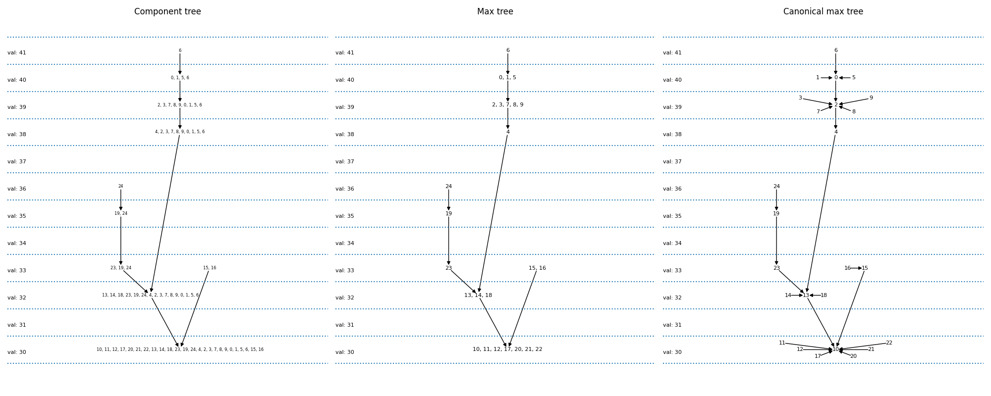
Max-treeのプロット

次に、コンポーネントツリーとMax-treeをプロットします。コンポーネントツリーは、すべての可能な閾値処理から生じる異なるピクセルセットを互いに関連付けます。あるレベルのコンポーネントが下位レベルのコンポーネントに含まれている場合、グラフには矢印があります。Max-treeは、ピクセルセットの異なるエンコーディングにすぎません。

1. コンポーネントツリー：ピクセルセットは明示的に書き出されます。たとえば、{6}（41で閾値処理を適用した結果）は、{0, 1, 5, 6}（40で閾値処理した結果）の親であることがわかります。

2. Max-tree：このレベルでセットに入るピクセルのみが明示的に書き出されます。したがって、{6} -> {0,1,5,6}の代わりに{6} -> {0,1,5}と書きます。

3. 標準Max-tree：これは、実装によって提供される表現です。ここでは、すべてのピクセルがノードです。複数のピクセルの連結成分は、ピクセルの1つで表されます。したがって、{6} -> {0,1,5}を{6} -> {5}、{1} -> {5}、{0} -> {5}に置き換えます。これにより、グラフを画像（上段、3列目）で表現できます。

# the canonical max-tree graph
canonical_max_tree = nx.DiGraph()
canonical_max_tree.add_nodes_from(S)
for node in canonical_max_tree.nodes():
    canonical_max_tree.nodes[node]['value'] = image_rav[node]
canonical_max_tree.add_edges_from([(n, P_rav[n]) for n in S[1:]])

# max-tree from the canonical max-tree
nx_max_tree = nx.DiGraph(canonical_max_tree)
labels = {}
prune(nx_max_tree, S[0], labels)

# component tree from the max-tree
labels_ct = {}
total = accumulate(nx_max_tree, S[0], labels_ct)

# positions of nodes : canonical max-tree (CMT)
pos_cmt = position_nodes_for_max_tree(canonical_max_tree, image_rav)

# positions of nodes : max-tree (MT)
pos_mt = dict(zip(nx_max_tree.nodes, [pos_cmt[node] for node in nx_max_tree.nodes]))

# plot the trees with networkx and matplotlib
fig, (ax1, ax2, ax3) = plt.subplots(1, 3, sharey=True, figsize=(20, 8))

plot_tree(
    nx_max_tree,
    pos_mt,
    ax1,
    title='Component tree',
    labels=labels_ct,
    font_size=6,
    text_size=8,
)

plot_tree(nx_max_tree, pos_mt, ax2, title='Max tree', labels=labels)

plot_tree(canonical_max_tree, pos_cmt, ax3, title='Canonical max tree')

fig.tight_layout()

plt.show()