注
最後の部分に移動して、完全なサンプルコードをダウンロードするか、Binderを介してブラウザでこの例を実行してください。
Liの閾値処理#
1993年、LiとLeeは、画像の背景と前景を区別するための「最適な」閾値を見つけるための新しい基準を提案しました[1]。彼らは、前景と前景平均、および背景と背景平均との間のクロスエントロピーを最小化すると、ほとんどの場合、最適な閾値が得られると提案しました。
ただし、1998年まで、この閾値を見つける方法は、可能なすべての閾値を試してから、クロスエントロピーが最小になるものを選択することでした。その時点で、LiとTamは、クロスエントロピーの傾きを使用して最適な点をより迅速に見つけるための新しい反復法を実装しました[2]。これは、scikit-imageのskimage.filters.threshold_li()で実装されている方法です。
ここでは、Liの反復法によるクロスエントロピーとその最適化について説明します。プライベート関数_cross_entropyを使用していることに注意してください。これは変更される可能性があるため、本番環境のコードでは使用しないでください。
import numpy as np
import matplotlib.pyplot as plt
from skimage import data
from skimage import filters
from skimage.filters.thresholding import _cross_entropy

cell = data.cell()
camera = data.camera()
まず、skimage.data.camera()画像のすべての可能な閾値でのクロスエントロピーをプロットしてみましょう。
thresholds = np.arange(np.min(camera) + 1.5, np.max(camera) - 1.5)
entropies = [_cross_entropy(camera, t) for t in thresholds]

optimal_camera_threshold = thresholds[np.argmin(entropies)]

fig, ax = plt.subplots(1, 3, figsize=(8, 3))

ax[0].imshow(camera, cmap='gray')
ax[0].set_title('image')
ax[0].set_axis_off()

ax[1].imshow(camera > optimal_camera_threshold, cmap='gray')
ax[1].set_title('thresholded')
ax[1].set_axis_off()

ax[2].plot(thresholds, entropies)
ax[2].set_xlabel('thresholds')
ax[2].set_ylabel('cross-entropy')
ax[2].vlines(
    optimal_camera_threshold,
    ymin=np.min(entropies) - 0.05 * np.ptp(entropies),
    ymax=np.max(entropies) - 0.05 * np.ptp(entropies),
)
ax[2].set_title('optimal threshold')

fig.tight_layout()

print('The brute force optimal threshold is:', optimal_camera_threshold)
print('The computed optimal threshold is:', filters.threshold_li(camera))

plt.show()
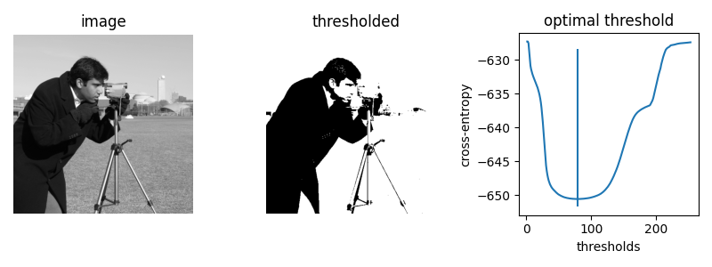
The brute force optimal threshold is: 78.5
The computed optimal threshold is: 78.91288426606151
次に、threshold_liのiter_callback機能を使用して、最適化プロセスを調べます。
iter_thresholds = []

optimal_threshold = filters.threshold_li(camera, iter_callback=iter_thresholds.append)
iter_entropies = [_cross_entropy(camera, t) for t in iter_thresholds]

print('Only', len(iter_thresholds), 'thresholds examined.')

fig, ax = plt.subplots()

ax.plot(thresholds, entropies, label='all threshold entropies')
ax.plot(iter_thresholds, iter_entropies, label='optimization path')
ax.scatter(iter_thresholds, iter_entropies, c='C1')
ax.legend(loc='upper right')

plt.show()
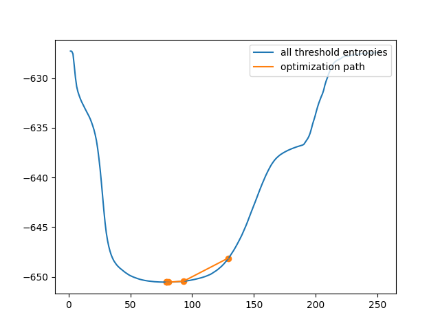
Only 5 thresholds examined.
これは明らかに、総当り法よりもはるかに効率的です。ただし、一部の画像では、クロスエントロピーは凸ではありません。つまり、単一の最適値を持つことを意味します。この場合、勾配降下法では、最適ではない閾値が得られる可能性があります。この例では、最適化の初期推定が不適切であると、閾値の選択が不十分になる様子を示します。
iter_thresholds2 = []

opt_threshold2 = filters.threshold_li(
    cell, initial_guess=64, iter_callback=iter_thresholds2.append
)

thresholds2 = np.arange(np.min(cell) + 1.5, np.max(cell) - 1.5)
entropies2 = [_cross_entropy(cell, t) for t in thresholds]
iter_entropies2 = [_cross_entropy(cell, t) for t in iter_thresholds2]

fig, ax = plt.subplots(1, 3, figsize=(8, 3))

ax[0].imshow(cell, cmap='magma')
ax[0].set_title('image')
ax[0].set_axis_off()

ax[1].imshow(cell > opt_threshold2, cmap='gray')
ax[1].set_title('thresholded')
ax[1].set_axis_off()

ax[2].plot(thresholds2, entropies2, label='all threshold entropies')
ax[2].plot(iter_thresholds2, iter_entropies2, label='optimization path')
ax[2].scatter(iter_thresholds2, iter_entropies2, c='C1')
ax[2].legend(loc='upper right')

plt.show()
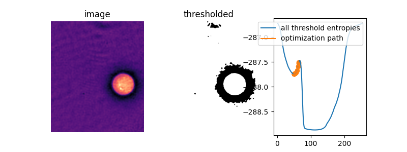
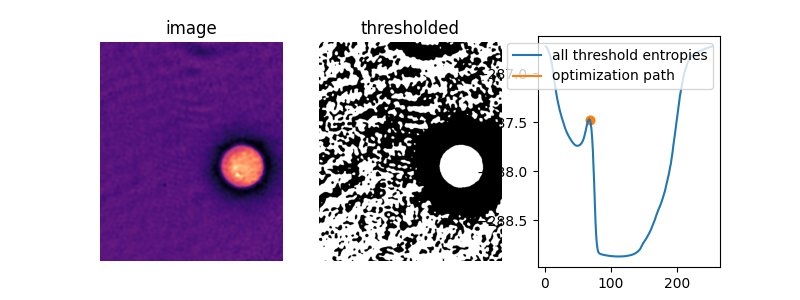
この画像では、驚くべきことに、デフォルトの初期推定である平均画像値が、実際には目的関数の2つの「谷」の間のピークの真上にあります。初期推定値を指定しないと、Liの閾値処理方法はまったく何も行いません!
iter_thresholds3 = []

opt_threshold3 = filters.threshold_li(cell, iter_callback=iter_thresholds3.append)

iter_entropies3 = [_cross_entropy(cell, t) for t in iter_thresholds3]

fig, ax = plt.subplots(1, 3, figsize=(8, 3))

ax[0].imshow(cell, cmap='magma')
ax[0].set_title('image')
ax[0].set_axis_off()

ax[1].imshow(cell > opt_threshold3, cmap='gray')
ax[1].set_title('thresholded')
ax[1].set_axis_off()

ax[2].plot(thresholds2, entropies2, label='all threshold entropies')
ax[2].plot(iter_thresholds3, iter_entropies3, label='optimization path')
ax[2].scatter(iter_thresholds3, iter_entropies3, c='C1')
ax[2].legend(loc='upper right')

plt.show()
何が起こっているかを確認するために、Liメソッドの内部ループを複製し、現在の閾値から次の閾値への変化を返す関数li_gradientを定義しましょう。この勾配が0の場合、いわゆる停留点にあり、Liはこの値を返します。負の場合、次の閾値の推定値は小さくなり、正の場合、次の推定値は大きくなります。
下のプロットでは、初期推定値がそのエントロピーピークの右側にある場合のクロスエントロピーとLiの更新パスを示します。閾値更新勾配を重ね合わせ、0勾配線とthreshold_liによるデフォルトの初期推定値をマークします。
def li_gradient(image, t):
    """Find the threshold update at a given threshold."""
    foreground = image > t
    mean_fore = np.mean(image[foreground])
    mean_back = np.mean(image[~foreground])
    t_next = (mean_back - mean_fore) / (np.log(mean_back) - np.log(mean_fore))
    dt = t_next - t
    return dt


iter_thresholds4 = []
opt_threshold4 = filters.threshold_li(
    cell, initial_guess=68, iter_callback=iter_thresholds4.append
)
iter_entropies4 = [_cross_entropy(cell, t) for t in iter_thresholds4]
print(len(iter_thresholds4), 'examined, optimum:', opt_threshold4)

gradients = [li_gradient(cell, t) for t in thresholds2]

fig, ax1 = plt.subplots()
ax1.plot(thresholds2, entropies2)
ax1.plot(iter_thresholds4, iter_entropies4)
ax1.scatter(iter_thresholds4, iter_entropies4, c='C1')
ax1.set_xlabel('threshold')
ax1.set_ylabel('cross entropy', color='C0')
ax1.tick_params(axis='y', labelcolor='C0')

ax2 = ax1.twinx()
ax2.plot(thresholds2, gradients, c='C3')
ax2.hlines(
    [0], xmin=thresholds2[0], xmax=thresholds2[-1], colors='gray', linestyles='dashed'
)
ax2.vlines(
    np.mean(cell),
    ymin=np.min(gradients),
    ymax=np.max(gradients),
    colors='gray',
    linestyles='dashed',
)
ax2.set_ylabel(r'$\Delta$(threshold)', color='C3')
ax2.tick_params(axis='y', labelcolor='C3')

fig.tight_layout()

plt.show()
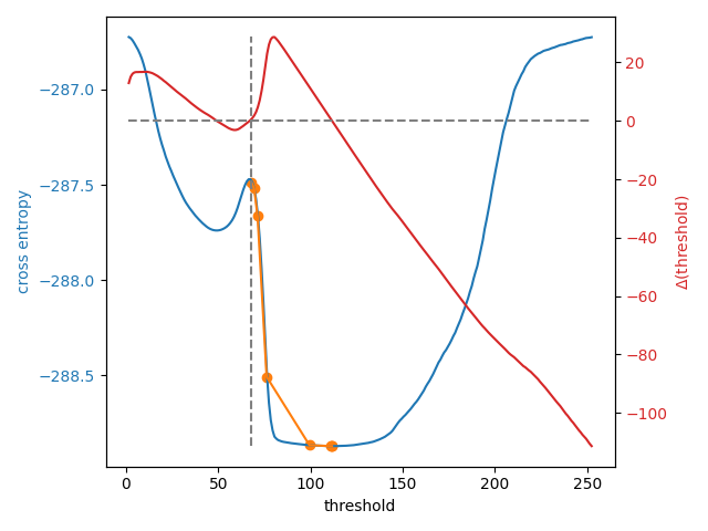
8 examined, optimum: 111.68876119648344
初期推定として数値を提供できるようにすることに加えて、skimage.filters.threshold_li()は、numpy.mean()がデフォルトで行うように、画像強度から推定を行う関数を受け取ることができます。これは、さまざまな範囲を持つ多くの画像を処理する必要がある場合に適したオプションとなる可能性があります。
def quantile_95(image):
    # you can use np.quantile(image, 0.95) if you have NumPy>=1.15
    return np.percentile(image, 95)


iter_thresholds5 = []
opt_threshold5 = filters.threshold_li(
    cell, initial_guess=quantile_95, iter_callback=iter_thresholds5.append
)
iter_entropies5 = [_cross_entropy(cell, t) for t in iter_thresholds5]
print(len(iter_thresholds5), 'examined, optimum:', opt_threshold5)

fig, ax1 = plt.subplots()
ax1.plot(thresholds2, entropies2)
ax1.plot(iter_thresholds5, iter_entropies5)
ax1.scatter(iter_thresholds5, iter_entropies5, c='C1')
ax1.set_xlabel('threshold')
ax1.set_ylabel('cross entropy', color='C0')
ax1.tick_params(axis='y', labelcolor='C0')

plt.show()
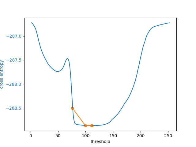
5 examined, optimum: 111.68876119648344
スクリプトの総実行時間:(0分5.120秒)