スライドウィンドウヒストグラム

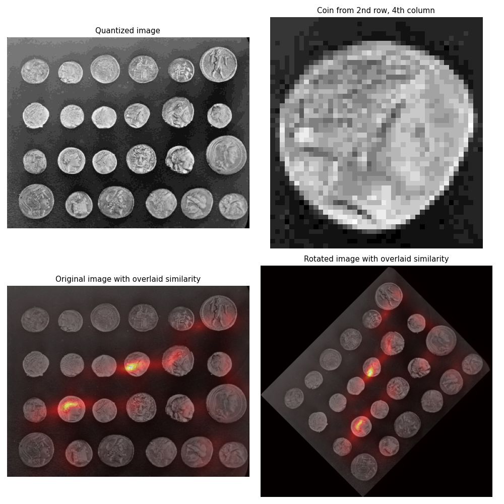
ヒストグラムマッチングは、画像内のオブジェクト検出に使用できます [1]。この例では、skimage.data.coins 画像から単一のコインを抽出し、ヒストグラムマッチングを使用して元の画像内での位置を特定しようとします。

まず、ターゲットコインを含む画像の箱形の領域が抽出され、そのグレースケール値のヒストグラムが計算されます。

次に、テスト画像の各ピクセルについて、ピクセルを囲む画像領域のグレースケール値のヒストグラムが計算されます。 skimage.filters.rank.windowed_histogram は、これらのヒストグラムを高速に計算できる効率的なスライドウィンドウベースのアルゴリズムを採用しているため、このタスクに使用されます [2]。画像内の各ピクセルを囲む領域の局所ヒストグラムは、単一のコインのヒストグラムと比較され、類似度尺度が計算されて表示されます。

単一のコインのヒストグラムは、コインを囲む箱形の領域で numpy.histogram を使用して計算されます。一方、スライドウィンドウヒストグラムは、わずかに異なるサイズの円盤状の構造化要素を使用して計算されます。これは、これらの違いがあっても、この手法が依然として類似性を見つけることを示すために実施されます。

この手法の回転不変性を示すために、45度回転させたコイン画像のバージョンで同じテストが実行されます。

参考文献

[1]

Porikli, F. “Integral Histogram: A Fast Way to Extract Histograms in Cartesian Spaces” CVPR, 2005. Vol. 1. IEEE, 2005

[2]

S.Perreault and P.Hebert. Median filtering in constant time. Trans. Image Processing, 16(9):2389-2394, 2007.

import numpy as np
import matplotlib
import matplotlib.pyplot as plt

from skimage import data, transform
from skimage.util import img_as_ubyte
from skimage.morphology import disk
from skimage.filters import rank


matplotlib.rcParams['font.size'] = 9


def windowed_histogram_similarity(image, footprint, reference_hist, n_bins):
    # Compute normalized windowed histogram feature vector for each pixel
    px_histograms = rank.windowed_histogram(image, footprint, n_bins=n_bins)

    # Reshape coin histogram to (1,1,N) for broadcast when we want to use it in
    # arithmetic operations with the windowed histograms from the image
    reference_hist = reference_hist.reshape((1, 1) + reference_hist.shape)

    # Compute Chi squared distance metric: sum((X-Y)^2 / (X+Y));
    # a measure of distance between histograms
    X = px_histograms
    Y = reference_hist

    num = (X - Y) ** 2
    denom = X + Y
    denom[denom == 0] = np.inf
    frac = num / denom

    chi_sqr = 0.5 * np.sum(frac, axis=2)

    # Generate a similarity measure. It needs to be low when distance is high
    # and high when distance is low; taking the reciprocal will do this.
    # Chi squared will always be >= 0, add small value to prevent divide by 0.
    similarity = 1 / (chi_sqr + 1.0e-4)

    return similarity


# Load the `skimage.data.coins` image
img = img_as_ubyte(data.coins())

# Quantize to 16 levels of grayscale; this way the output image will have a
# 16-dimensional feature vector per pixel
quantized_img = img // 16

# Select the coin from the 4th column, second row.
# Coordinate ordering: [x1,y1,x2,y2]
coin_coords = [184, 100, 228, 148]  # 44 x 44 region
coin = quantized_img[coin_coords[1] : coin_coords[3], coin_coords[0] : coin_coords[2]]

# Compute coin histogram and normalize
coin_hist, _ = np.histogram(coin.flatten(), bins=16, range=(0, 16))
coin_hist = coin_hist.astype(float) / np.sum(coin_hist)

# Compute a disk shaped mask that will define the shape of our sliding window
# Example coin is ~44px across, so make a disk 61px wide (2 * rad + 1) to be
# big enough for other coins too.
footprint = disk(30)

# Compute the similarity across the complete image
similarity = windowed_histogram_similarity(
    quantized_img, footprint, coin_hist, coin_hist.shape[0]
)

# Now try a rotated image
rotated_img = img_as_ubyte(transform.rotate(img, 45.0, resize=True))
# Quantize to 16 levels as before
quantized_rotated_image = rotated_img // 16
# Similarity on rotated image
rotated_similarity = windowed_histogram_similarity(
    quantized_rotated_image, footprint, coin_hist, coin_hist.shape[0]
)

fig, axes = plt.subplots(nrows=2, ncols=2, figsize=(10, 10))

axes[0, 0].imshow(quantized_img, cmap='gray')
axes[0, 0].set_title('Quantized image')
axes[0, 0].axis('off')

axes[0, 1].imshow(coin, cmap='gray')
axes[0, 1].set_title('Coin from 2nd row, 4th column')
axes[0, 1].axis('off')

axes[1, 0].imshow(img, cmap='gray')
axes[1, 0].imshow(similarity, cmap='hot', alpha=0.5)
axes[1, 0].set_title('Original image with overlaid similarity')
axes[1, 0].axis('off')

axes[1, 1].imshow(rotated_img, cmap='gray')
axes[1, 1].imshow(rotated_similarity, cmap='hot', alpha=0.5)
axes[1, 1].set_title('Rotated image with overlaid similarity')
axes[1, 1].axis('off')

plt.tight_layout()
plt.show()