レジストレーションのための極座標変換とログ極座標変換の使用

位相相関（registration.phase_cross_correlation）は、類似した画像ペア間の並進オフセットを決定するための効率的な方法です。ただし、このアプローチは、画像間の回転/スケーリングの違いがほとんどないことに依存しており、これは現実世界の例では一般的です。

2つの画像間の回転とスケーリングの違いを復元するために、ログ極座標変換の2つの幾何学的特性と周波数領域の並進不変性を利用できます。まず、デカルト空間での回転は、ログ極座標空間の角度座標（\(\theta\)）軸に沿った並進になります。次に、デカルト空間でのスケーリングは、ログ極座標空間の半径座標（\(\rho = \ln\sqrt{x^2 + y^2}\)）に沿った並進になります。最後に、空間領域での並進の違いは、周波数領域での大きさスペクトルには影響しません。

この一連の例では、これらの概念に基づいて、ログ極座標変換transform.warp_polarを位相相関と組み合わせて使用して、並進オフセットも持つ2つの画像間の回転とスケーリングの違いを復元する方法を示します。

極座標変換による回転差の復元

最初の例では、共通の中心点を中心とした回転に関してのみ異なる2つの画像の簡単なケースを検討します。これらの画像を極座標空間に再マッピングすると、回転の差が位相相関によって復元できる単純な並進の差になります。

import numpy as np
import matplotlib.pyplot as plt

from skimage import data
from skimage.registration import phase_cross_correlation
from skimage.transform import warp_polar, rotate, rescale
from skimage.util import img_as_float

radius = 705
angle = 35
image = data.retina()
image = img_as_float(image)
rotated = rotate(image, angle)
image_polar = warp_polar(image, radius=radius, channel_axis=-1)
rotated_polar = warp_polar(rotated, radius=radius, channel_axis=-1)

fig, axes = plt.subplots(2, 2, figsize=(8, 8))
ax = axes.ravel()
ax[0].set_title("Original")
ax[0].imshow(image)
ax[1].set_title("Rotated")
ax[1].imshow(rotated)
ax[2].set_title("Polar-Transformed Original")
ax[2].imshow(image_polar)
ax[3].set_title("Polar-Transformed Rotated")
ax[3].imshow(rotated_polar)
plt.show()

shifts, error, phasediff = phase_cross_correlation(
    image_polar, rotated_polar, normalization=None
)
print(f'Expected value for counterclockwise rotation in degrees: ' f'{angle}')
print(f'Recovered value for counterclockwise rotation: ' f'{shifts[0]}')

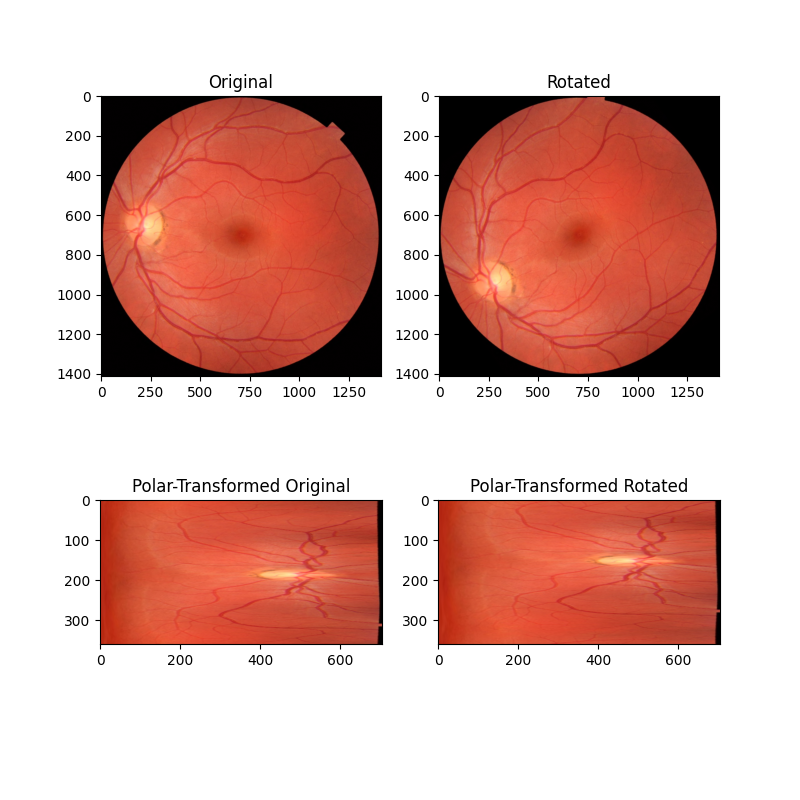
Expected value for counterclockwise rotation in degrees: 35
Recovered value for counterclockwise rotation: 35.0

ログ極座標変換による回転とスケーリングの違いの復元

この2番目の例では、画像は回転とスケーリングの両方で異なります（軸の目盛り値に注意してください）。これらの画像をログ極座標空間に再マッピングすることで、以前と同様に回転を復元し、位相相関によってスケーリングも復元できるようになりました。

# radius must be large enough to capture useful info in larger image
radius = 1500
angle = 53.7
scale = 2.2
image = data.retina()
image = img_as_float(image)
rotated = rotate(image, angle)
rescaled = rescale(rotated, scale, channel_axis=-1)
image_polar = warp_polar(image, radius=radius, scaling='log', channel_axis=-1)
rescaled_polar = warp_polar(rescaled, radius=radius, scaling='log', channel_axis=-1)

fig, axes = plt.subplots(2, 2, figsize=(8, 8))
ax = axes.ravel()
ax[0].set_title("Original")
ax[0].imshow(image)
ax[1].set_title("Rotated and Rescaled")
ax[1].imshow(rescaled)
ax[2].set_title("Log-Polar-Transformed Original")
ax[2].imshow(image_polar)
ax[3].set_title("Log-Polar-Transformed Rotated and Rescaled")
ax[3].imshow(rescaled_polar)
plt.show()

# setting `upsample_factor` can increase precision
shifts, error, phasediff = phase_cross_correlation(
    image_polar, rescaled_polar, upsample_factor=20, normalization=None
)
shiftr, shiftc = shifts[:2]

# Calculate scale factor from translation
klog = radius / np.log(radius)
shift_scale = 1 / (np.exp(shiftc / klog))

print(f'Expected value for cc rotation in degrees: {angle}')
print(f'Recovered value for cc rotation: {shiftr}')
print()
print(f'Expected value for scaling difference: {scale}')
print(f'Recovered value for scaling difference: {shift_scale}')

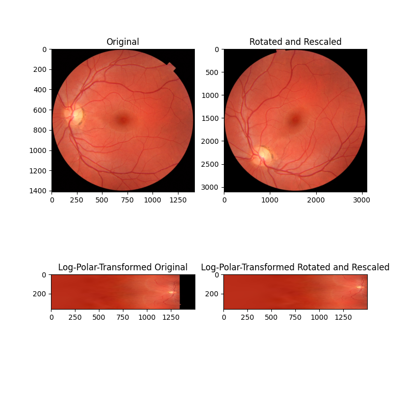
Expected value for cc rotation in degrees: 53.7
Recovered value for cc rotation: 53.75

Expected value for scaling difference: 2.2
Recovered value for scaling difference: 2.1981889915232165

並進された画像に対する回転とスケーリングの登録 - パート1

上記の例は、登録する画像が中心を共有する場合にのみ機能します。ただし、登録する2つの画像間の違いに並進成分がある場合の方が多くあります。回転、スケーリング、並進を登録する1つのアプローチは、最初に回転とスケーリングを修正してから、並進を解決することです。フーリエ変換された画像の大きさスペクトルを処理することで、並進された画像の回転とスケーリングの違いを解決できます。

次の例では、2つの画像が回転、スケーリング、並進で異なる場合、上記のアプローチがどのように失敗するかを最初に示します。

from skimage.color import rgb2gray
from skimage.filters import window, difference_of_gaussians
from scipy.fft import fft2, fftshift

angle = 24
scale = 1.4
shiftr = 30
shiftc = 15

image = rgb2gray(data.retina())
translated = image[shiftr:, shiftc:]
rotated = rotate(translated, angle)
rescaled = rescale(rotated, scale)
sizer, sizec = image.shape
rts_image = rescaled[:sizer, :sizec]

# When center is not shared, log-polar transform is not helpful!
radius = 705
warped_image = warp_polar(image, radius=radius, scaling="log")
warped_rts = warp_polar(rts_image, radius=radius, scaling="log")
shifts, error, phasediff = phase_cross_correlation(
    warped_image, warped_rts, upsample_factor=20, normalization=None
)
shiftr, shiftc = shifts[:2]
klog = radius / np.log(radius)
shift_scale = 1 / (np.exp(shiftc / klog))

fig, axes = plt.subplots(2, 2, figsize=(8, 8))
ax = axes.ravel()
ax[0].set_title("Original Image")
ax[0].imshow(image, cmap='gray')
ax[1].set_title("Modified Image")
ax[1].imshow(rts_image, cmap='gray')
ax[2].set_title("Log-Polar-Transformed Original")
ax[2].imshow(warped_image)
ax[3].set_title("Log-Polar-Transformed Modified")
ax[3].imshow(warped_rts)
fig.suptitle('log-polar-based registration fails when no shared center')
plt.show()

print(f'Expected value for cc rotation in degrees: {angle}')
print(f'Recovered value for cc rotation: {shiftr}')
print()
print(f'Expected value for scaling difference: {scale}')
print(f'Recovered value for scaling difference: {shift_scale}')

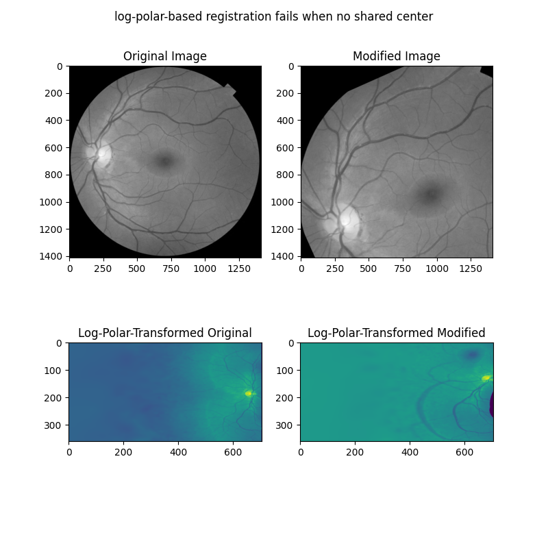
Expected value for cc rotation in degrees: 24
Recovered value for cc rotation: -167.55

Expected value for scaling difference: 1.4
Recovered value for scaling difference: 25.110458986143573

並進された画像に対する回転とスケーリングの登録 - パート2

次に、並進の違いではなく、回転とスケーリングの違いが画像の周波数振幅スペクトルでどのように明らかになるかを示します。これらの違いは、大きさスペクトルを画像自体として扱い、上記と同様のログ極座標+位相相関アプローチを適用することで復元できます。

# First, band-pass filter both images
image = difference_of_gaussians(image, 5, 20)
rts_image = difference_of_gaussians(rts_image, 5, 20)

# window images
wimage = image * window('hann', image.shape)
rts_wimage = rts_image * window('hann', image.shape)

# work with shifted FFT magnitudes
image_fs = np.abs(fftshift(fft2(wimage)))
rts_fs = np.abs(fftshift(fft2(rts_wimage)))

# Create log-polar transformed FFT mag images and register
shape = image_fs.shape
radius = shape[0] // 8  # only take lower frequencies
warped_image_fs = warp_polar(
    image_fs, radius=radius, output_shape=shape, scaling='log', order=0
)
warped_rts_fs = warp_polar(
    rts_fs, radius=radius, output_shape=shape, scaling='log', order=0
)

warped_image_fs = warped_image_fs[: shape[0] // 2, :]  # only use half of FFT
warped_rts_fs = warped_rts_fs[: shape[0] // 2, :]
shifts, error, phasediff = phase_cross_correlation(
    warped_image_fs, warped_rts_fs, upsample_factor=10, normalization=None
)

# Use translation parameters to calculate rotation and scaling parameters
shiftr, shiftc = shifts[:2]
recovered_angle = (360 / shape[0]) * shiftr
klog = shape[1] / np.log(radius)
shift_scale = np.exp(shiftc / klog)

fig, axes = plt.subplots(2, 2, figsize=(8, 8))
ax = axes.ravel()
ax[0].set_title("Original Image FFT\n(magnitude; zoomed)")
center = np.array(shape) // 2
ax[0].imshow(
    image_fs[
        center[0] - radius : center[0] + radius, center[1] - radius : center[1] + radius
    ],
    cmap='magma',
)
ax[1].set_title("Modified Image FFT\n(magnitude; zoomed)")
ax[1].imshow(
    rts_fs[
        center[0] - radius : center[0] + radius, center[1] - radius : center[1] + radius
    ],
    cmap='magma',
)
ax[2].set_title("Log-Polar-Transformed\nOriginal FFT")
ax[2].imshow(warped_image_fs, cmap='magma')
ax[3].set_title("Log-Polar-Transformed\nModified FFT")
ax[3].imshow(warped_rts_fs, cmap='magma')
fig.suptitle('Working in frequency domain can recover rotation and scaling')
plt.show()

print(f'Expected value for cc rotation in degrees: {angle}')
print(f'Recovered value for cc rotation: {recovered_angle}')
print()
print(f'Expected value for scaling difference: {scale}')
print(f'Recovered value for scaling difference: {shift_scale}')

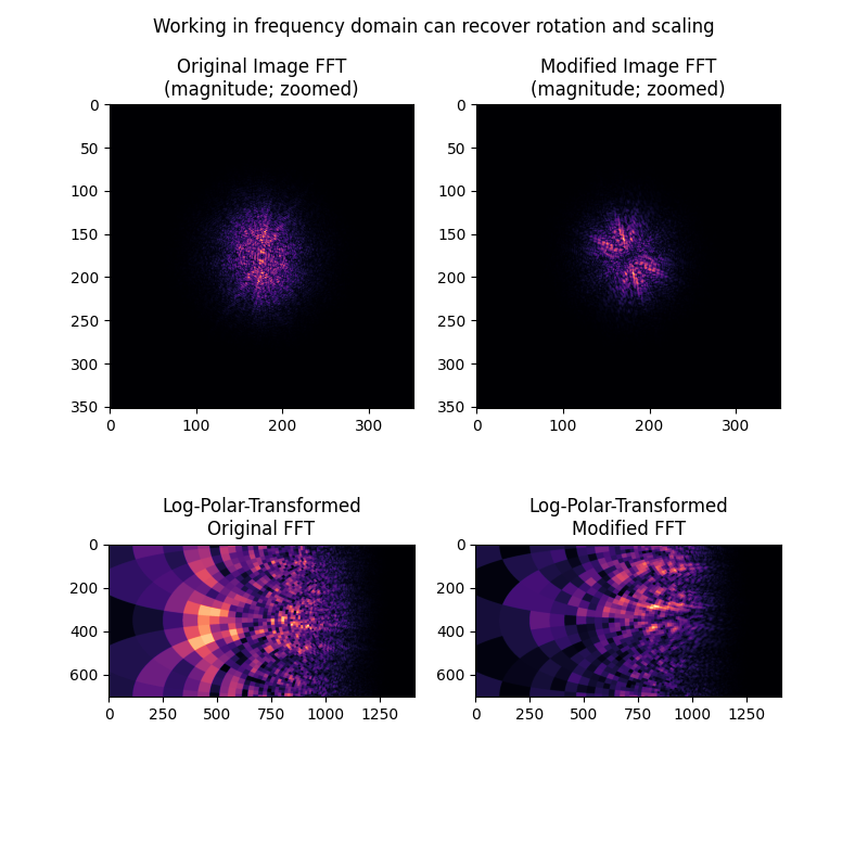
Expected value for cc rotation in degrees: 24
Recovered value for cc rotation: 23.753366406803682

Expected value for scaling difference: 1.4
Recovered value for scaling difference: 1.3901762721757436

このアプローチに関するいくつかの注意点

このアプローチは、事前に選択する必要があり、明確に最適な選択がないいくつかのパラメーターに依存していることに注意する必要があります。

1. 画像には、特に高周波を除去するために、ある程度のバンドパスフィルタリングを適用する必要があり、ここでの選択の違いが結果に影響を与える可能性があります。バンドパスフィルターは、登録する画像のスケールが異なり、これらのスケールの違いが不明であるため、バンドパスフィルターは必然的に画像間で異なる特徴を減衰させるため、問題を複雑にします。たとえば、ここで最後の例では、ログ極座標変換された大きさスペクトルは実際には「似ている」ようには見えません。ただし、よく見ると、それらのスペクトルにはいくつかの共通のパターンがあり、示されているように位相相関によってうまく整列します。

2. 画像の境界から来るスペクトル漏れを除去するために、円対称性を持つ窓を使用して画像を窓化する必要があります。窓の明確に最適な選択はありません。

最後に、スケールの大きな変更は、特にスケールの大きな変更が通常、一部の切り抜きや情報量の損失を伴うため、マグニチュードスペクトルを劇的に変化させることに注意してください。文献では、1.8〜2倍のスケール変更内に留まることが推奨されています[1] [2]。これは、ほとんどの生物学的画像処理アプリケーションでは問題ありません。

参考文献

[1]

B.S. Reddy and B.N. Chatterji. An FFT-based technique for translation, rotation and scale- invariant image registration. IEEE Trans. Image Processing, 5(8):1266–1271, 1996. DOI:10.1109/83.506761

[2]

Tzimiropoulos, Georgios, and Tania Stathaki. “Robust FFT-based scale-invariant image registration.” In 4th SEAS DTC Technical Conference. 2009. DOI:10.1109/TPAMI.2010.107