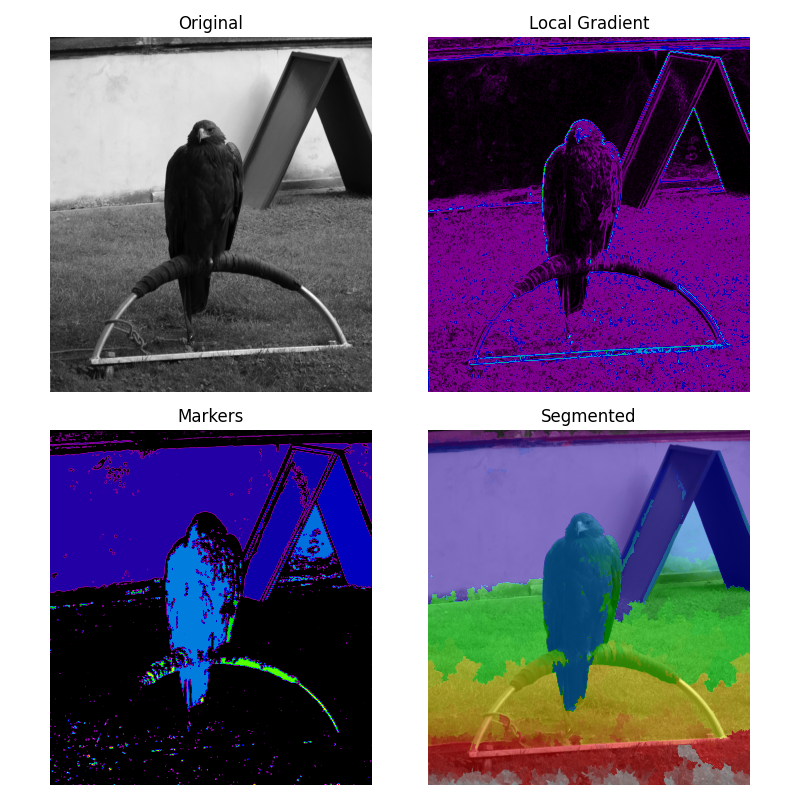
ウォーターシェッド変換のマーカー

ウォーターシェッドは、セグメンテーション、つまり画像内の異なるオブジェクトを分離するために使用される古典的なアルゴリズムです。

ここでは、画像内の低勾配領域からマーカー画像が構築されます。勾配画像では、値の高い領域が画像のセグメント化に役立つ障壁を提供します。低い値にマーカーを使用することで、セグメント化されたオブジェクトが確実に見つかります。

アルゴリズムの詳細は、Wikipediaを参照してください。

from scipy import ndimage as ndi
import matplotlib.pyplot as plt

from skimage.morphology import disk
from skimage.segmentation import watershed
from skimage import data
from skimage.filters import rank
from skimage.util import img_as_ubyte


image = img_as_ubyte(data.eagle())

# denoise image
denoised = rank.median(image, disk(2))

# find continuous region (low gradient -
# where less than 10 for this image) --> markers
# disk(5) is used here to get a more smooth image
markers = rank.gradient(denoised, disk(5)) < 10
markers = ndi.label(markers)[0]

# local gradient (disk(2) is used to keep edges thin)
gradient = rank.gradient(denoised, disk(2))

# process the watershed
labels = watershed(gradient, markers)

# display results
fig, axes = plt.subplots(nrows=2, ncols=2, figsize=(8, 8), sharex=True, sharey=True)
ax = axes.ravel()

ax[0].imshow(image, cmap=plt.cm.gray)
ax[0].set_title("Original")

ax[1].imshow(gradient, cmap=plt.cm.nipy_spectral)
ax[1].set_title("Local Gradient")

ax[2].imshow(markers, cmap=plt.cm.nipy_spectral)
ax[2].set_title("Markers")

ax[3].imshow(image, cmap=plt.cm.gray)
ax[3].imshow(labels, cmap=plt.cm.nipy_spectral, alpha=0.5)
ax[3].set_title("Segmented")

for a in ax:
    a.axis('off')

fig.tight_layout()
plt.show()